
Background
Backpropagation is a common method for training a neural network. There is no shortage of papers online that attempt to explain how backpropagation works, but few that include an example with actual numbers. This post is my attempt to explain how it works with a concrete example that folks can compare their own calculations to in order to ensure they understand backpropagation correctly.
Backpropagation in Python
You can play around with a Python script that I wrote that implements the backpropagation algorithm in this Github repo.
Continue learning with Emergent Mind
If you find this tutorial useful and want to continue learning about AI/ML, I encourage you to check out Emergent Mind, a new website I’m working on that uses GPT-4 to surface and explain cutting-edge AI/ML papers:

In time, I hope to use AI to explain complex AI/ML topics on Emergent Mind in a style similar to what you’ll find in the tutorial below.
Now, on with the backpropagation tutorial…
Overview
For this tutorial, we’re going to use a neural network with two inputs, two hidden neurons, two output neurons. Additionally, the hidden and output neurons will include a bias.
Here’s the basic structure:

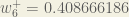
In order to have some numbers to work with, here are the initial weights, the biases, and training inputs/outputs:
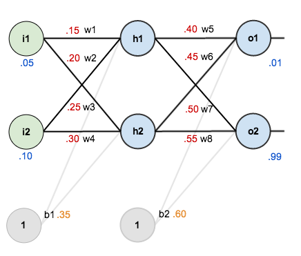
The goal of backpropagation is to optimize the weights so that the neural network can learn how to correctly map arbitrary inputs to outputs.
For the rest of this tutorial we’re going to work with a single training set: given inputs 0.05 and 0.10, we want the neural network to output 0.01 and 0.99.
The Forward Pass
To begin, lets see what the neural network currently predicts given the weights and biases above and inputs of 0.05 and 0.10. To do this we’ll feed those inputs forward though the network.
We figure out the total net input to each hidden layer neuron, squash the total net input using an activation function (here we use the logistic function), then repeat the process with the output layer neurons.
Here’s how we calculate the total net input for 


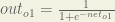
We then squash it using the logistic function to get the output of

Carrying out the same process for 
We repeat this process for the output layer neurons, using the output from the hidden layer neurons as inputs.
Here’s the output for 


And carrying out the same process for 

Calculating the Total Error
We can now calculate the error for each output neuron using the squared error function and sum them to get the total error:

 is included so that exponent is cancelled when we differentiate later on. The result is eventually multiplied by a learning rate anyway so it doesn’t matter that we introduce a constant here [1].
For example, the target output for

Repeating this process for 
The total error for the neural network is the sum of these errors:

The Backwards Pass
Our goal with backpropagation is to update each of the weights in the network so that they cause the actual output to be closer the target output, thereby minimizing the error for each output neuron and the network as a whole.
Output Layer
Consider 

 is read as “the partial derivative of
  with respect to
  “. You can also say “the gradient with respect to ”.
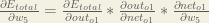
By applying the chain rule we know that:

Visually, here’s what we’re doing:

We need to figure out each piece in this equation.
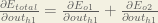
First, how much does the total error change with respect to the output?


When we take the partial derivative of the total error with respect to 

Next, how much does the output of
The partial derivative of the logistic function is the output multiplied by 1 minus the output:

Finally, how much does the total net input of 

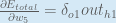
Putting it all together:

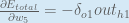
You’ll often see this calculation combined in the form of the delta rule:

Alternatively, we have 


Therefore:
Some sources extract the negative sign from 
To decrease the error, we then subtract this value from the current weight (optionally multiplied by some learning rate, eta, which we’ll set to 0.5):

 (alpha) to represent the learning rate, others use
  (eta), and others even use
  (epsilon).
We can repeat this process to get the new weights 


We perform the actual updates in the neural network after we have the new weights leading into the hidden layer neurons (ie, we use the original weights, not the updated weights, when we continue the backpropagation algorithm below).
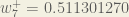
Hidden Layer
Next, we’ll continue the backwards pass by calculating new values for 


Big picture, here’s what we need to figure out:

Visually:
We’re going to use a similar process as we did for the output layer, but slightly different to account for the fact that the output of each hidden layer neuron contributes to the output (and therefore error) of multiple output neurons. We know that 


Starting with 
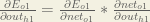
We can calculate 

And 

Plugging them in:

Following the same process for 
Therefore:

Now that we have 


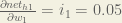
We calculate the partial derivative of the total net input to

Putting it all together:

You might also see this written as:


We can now update

Repeating this for


Finally, we’ve updated all of our weights! When we fed forward the 0.05 and 0.1 inputs originally, the error on the network was 0.298371109. After this first round of backpropagation, the total error is now down to 0.291027924. It might not seem like much, but after repeating this process 10,000 times, for example, the error plummets to 0.0000351085. At this point, when we feed forward 0.05 and 0.1, the two outputs neurons generate 0.015912196 (vs 0.01 target) and 0.984065734 (vs 0.99 target).
If you’ve made it this far and found any errors in any of the above or can think of any ways to make it clearer for future readers, don’t hesitate to drop me a note. Thanks!
And while I have you…
Again, if you liked this tutorial, please check out Emergent Mind, a site I’m building with an end goal of explaining AI/ML concepts in a similar style as this post. Feedback very much welcome!

Why are you calculating net_h1 with w1 and w2 instead of w1 and w3, which are the weights leading to h1?
You must take a closer look! net_h1 is connected with w1 and w3!
w2 and w3 are the names of the lines left, not for the lines right ;-)
You are correct. But, in the calculation of the net input h1, he uses the value of the weight w2 which is 0.2. The value for w3 is 0.25 and therefore the calculation of the net input of h1 should be:
h1 = 0.15 * 0.05 + 0.25 * 0.1 + 0.35
I hope it is correct.
I think you are correct. The weights are switched in his calculations.
Thanks matt, this blog help me learn a lot
excellent!!
Very intuitive and excellent.
There is a wrong value for ‘target o1’ when calculating ‘E o1.’ You are using 0.01 instead of 0.1, according to this picture https://matthewmazur.files.wordpress.com/2018/03/neural_network-9.png
thanks for the super great explaination
What to do with the bias ? Or will it have an initial random value forever ?
bias also must be updated
The best explanation!
This is great
Thanks a ton for this!
Thank you very much sir!
VThank you
Excellent post.
Many people evade the dirty calculations of back-propagation and tend to just mention it verbally and not with writing equations like you did, that being said, well done!
Hey,
That’s a very nice blog. How can we adapt the code to use mini-batch insteed of online learning? I have some problems with adaptations. Can someone help me out ?
Thanks
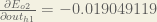
Shouldn’t the dE02/dOutH1 =-0.019049119 actually be = -0,01714420647497980579542508125?? Regards Morgan
Hallo guys,
Thanks you Matt for this great job.
can someone help me out to adapt this code so that it uses mini batch insteed of online learning ?
Thanks.
Great demo !
I wanted to check any details so i tried to implement it on Google Colab with tensorflow and Keras and i checked any line , any detail … i get the sames values for these 2 backpropagations on all parameters , weights , gradients , losses … check my link : check my link https://colab.research.google.com/drive/13i8YefcJfOo4Sg6QseER-AYwBUKQDl15?usp=sharing
Of course it can be presented a better way
best one
This post was useful in 2017 and is the best post about NNs in 2024. Truly world changing!
Great work indeed!!!
Good Work, we must appreciate this effort.
Very good explanation. This blog was the go to place when I was implementing a back propagation function in dart.
One suggestion I have is to abstract the derivative of the activation function and of the cost function, maybe with examples of alternative functions (ReLU, Huber loss, …) so that the modular feeling of training a NN is highlighted.
There’s a misleading mistake at the beginning. net_h1 calculation should use w1 and w3 but you use w1 and w2 so all the calculations are wrong.
Hy Paul
The calculation is as follow :
net H1 = w1 * i1 +w2 * i2 = 0.3375
w1= 0.15 , w2 = 0.20
i1 = 0.05 , i2 = 0.10 , b1 = 0.35
I checked all in a Python notebook where each step is checked and validated with the formulas. All formulas are correct.
net H1 = w1 * i1 +w2 * i2 = 0.3375
net H1 = w1 * i1 +w2 * i2 + b1 = 0.3375
Thank you 😊
i need same example but computing error with cross entropy..do you have it?
As mentioned earlier, bias is never updated in your calculations. I believe for a given layer:
new bias for a layer = old bias – training rate * the sum of dEtotal/dOut for all nodes in a layer.
So for the output layer:
dEtotal_wrt_dOut = dEo1_wrt_dOutO1 + dEo2_wrt_dOutO2
dEo1_wrt_dOutO1 = 0.7413650695523157
dEo2_wrt_dOutO2 = -0.21707153467853746
So dEtotal_wrt_dOut=0.5242935348737783
And therefore
new_b2 = old_b2(0.60) – training_rate(0.5) * dEtotal_wrt_dOut(0.5242935348737783)
= 0.33785323256311084
And for the hidden layer:
new_b1 = old_b1(0.35)-trainingRate(0.5)*dEtotal_wrt_dOut(0.0777206290418894)= 0.3111396854790553
By updating the bias, your solution will converge faster. My notation is a little wonky, but I love your article.
Great example. Searched at least 20-25 blogs for a step by step example before seeing your blog.
Matt isn’t calculating gradients for the Biases. So his answer is correct is you don’t touch the Biases. My code calculates gradients for biases and adjusts the biases during backprop, took me hours of debugging to figure out my code is correct …
<tthe correct way is your approach. the interation of the biases should als o be calculated. I guess after 10.000 itrations the loss should be better?
Is this corect Dan?
Das Ignorieren der Bias-Anpassungen während des Trainings ist im Allgemeinen ein Fehler, da es das Netzwerk in seiner Lernfähigkeit stark einschränkt. Nach sehr vielen Iterationen könnte sich das Ergebnis zwar stabilisieren, aber es wäre wahrscheinlich nicht optimal, und der Loss bliebe höher als bei einer vollständigen Anpassung der Gewichte und Biases. Um die besten Ergebnisse zu erzielen, sollten sowohl die Gewichte als auch die Biases in jeder Iteration aktualisiert werden.
why does he not calculate gradients for biases?
the biases shoud also like the weights be updated during each iteration…
The concept of attaching the biases in this blog is wrong. The biases should be attached to the input layer and the hidden layer (pyimagesearch.com). The blog is considering attaching the bias to the output.
This post is good only for students. Now that doesn’t help. I have on same database conducted an generative NN experiment. Starting from 1 neuron and 1 to 13 hidden layer to 400 neurons in each layer for 12 combinations of activation functions and solvers, generating more than 100 Gigs of data just to see how accuracy would change within changed hyperparameters. Now i can’t surpass 60%+ accuracy for known data on which it is tested. Those generative NN’s are hard to use and in most cases useless as majority can’t really use them. Artificial is the wrong word for it. More appropriate is DNN like “dumb” … Until there is no smart NN software developed which can adjust NN hypermeters in auto-corrective backwards way for for each instance tested based on % of required confidence of accuracy, this is like a fishing in a pond with no fish. Those achieved high accuracy rates posted all over the net are fake. Just like one can lie with % calculus u can easily lie with ANN. U make a prediction on some hyperparameters chosen and say your prediction is 97% accurate. Why? There is no way that someone can check and evaluate your hyperparameter’s – yet ! That’s why its so easy to lie and that’s the main reason why people can’t get the results out of it ! Even PhD-s at the end tells u, u should guess it in trial methods – good luck with that.
Matt, thanks a lot! Really helped to start! Mind – this model will never work with 16++ inputs. Weights should not be positive only. But anyway – Thank you for your Job!!!
T
Hello Matt, great demo! I just noticed that the weights of bias were not updated, that can also contribute to the reduction of the error. Best Greetings!
re the backwards propagation steps , why not simple
Greetings of the day,
sir please see the weight updation of w1 once, the differentiation of Eo1 with outh1 seems wrong.
Is there also a useful application example for this neuron network
Now that we have
, we need to figure out
and then
for each weight
I think ∂neth1 / ∂w above should be ∂neth1/∂w1