A Step by Step Backpropagation Example

March 17, 2015February 23, 2024Mazur

Background

Backpropagation is a common method for training a neural network. There is no shortage of papers online that attempt to explain how backpropagation works, but few that include an example with actual numbers. This post is my attempt to explain how it works with a concrete example that folks can compare their own calculations to in order to ensure they understand backpropagation correctly.

Backpropagation in Python

You can play around with a Python script that I wrote that implements the backpropagation algorithm in this Github repo.

Continue learning with Emergent Mind

If you find this tutorial useful and want to continue learning about AI/ML, I encourage you to check out Emergent Mind, a new website I’m working on that uses GPT-4 to surface and explain cutting-edge AI/ML papers:

In time, I hope to use AI to explain complex AI/ML topics on Emergent Mind in a style similar to what you’ll find in the tutorial below.

Now, on with the backpropagation tutorial…

Overview

For this tutorial, we’re going to use a neural network with two inputs, two hidden neurons, two output neurons. Additionally, the hidden and output neurons will include a bias.

Here’s the basic structure:

In order to have some numbers to work with, here are the initial weights, the biases, and training inputs/outputs:

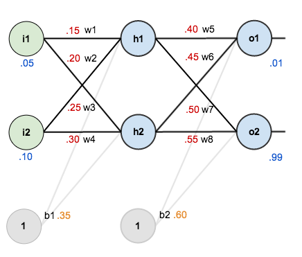
The goal of backpropagation is to optimize the weights so that the neural network can learn how to correctly map arbitrary inputs to outputs.

For the rest of this tutorial we’re going to work with a single training set: given inputs 0.05 and 0.10, we want the neural network to output 0.01 and 0.99.

The Forward Pass

To begin, lets see what the neural network currently predicts given the weights and biases above and inputs of 0.05 and 0.10. To do this we’ll feed those inputs forward though the network.

We figure out the total net input to each hidden layer neuron, squash the total net input using an activation function (here we use the logistic function), then repeat the process with the output layer neurons.

Total net input is also referred to as just net input by some sources.

Here’s how we calculate the total net input for $h_1$ :

$net_{h1} = w_1 * i_1 + w_2 * i_2 + b_1 * 1$

$net_{h1} = 0.15 * 0.05 + 0.2 * 0.1 + 0.35 * 1 = 0.3775$

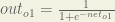
We then squash it using the logistic function to get the output of $h_1$ :

$out_{h1} = \frac{1}{1+e^{-net_{h1}}} = \frac{1}{1+e^{-0.3775}} = 0.593269992$

Carrying out the same process for $h_2$ we get:

$out_{h2} = 0.596884378$

We repeat this process for the output layer neurons, using the output from the hidden layer neurons as inputs.

Here’s the output for $o_1$ :

$net_{o1} = w_5 * out_{h1} + w_6 * out_{h2} + b_2 * 1$

$net_{o1} = 0.4 * 0.593269992 + 0.45 * 0.596884378 + 0.6 * 1 = 1.105905967$

$out_{o1} = \frac{1}{1+e^{-net_{o1}}} = \frac{1}{1+e^{-1.105905967}} = 0.75136507$

And carrying out the same process for $o_2$ we get:

$out_{o2} = 0.772928465$

Calculating the Total Error

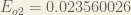
We can now calculate the error for each output neuron using the squared error function and sum them to get the total error:

$E_{total} = \sum \frac{1}{2}(target - output)^{2}$

Some sources refer to the target as the ideal and the output as the actual.

The $\frac{1}{2}$ is included so that exponent is cancelled when we differentiate later on. The result is eventually multiplied by a learning rate anyway so it doesn’t matter that we introduce a constant here [1].

For example, the target output for $o_1$ is 0.01 but the neural network output 0.75136507, therefore its error is:

$E_{o1} = \frac{1}{2}(target_{o1} - out_{o1})^{2} = \frac{1}{2}(0.01 - 0.75136507)^{2} = 0.274811083$

Repeating this process for $o_2$ (remembering that the target is 0.99) we get:

$E_{o2} = 0.023560026$

The total error for the neural network is the sum of these errors:

$E_{total} = E_{o1} + E_{o2} = 0.274811083 + 0.023560026 = 0.298371109$

The Backwards Pass

Our goal with backpropagation is to update each of the weights in the network so that they cause the actual output to be closer the target output, thereby minimizing the error for each output neuron and the network as a whole.

Output Layer

Consider $w_5$ . We want to know how much a change in $w_5$ affects the total error, aka $\frac{\partial E_{total}}{\partial w_{5}}$ .

$\frac{\partial E_{total}}{\partial w_{5}}$ is read as “the partial derivative of $E_{total}$ with respect to $w_{5}$ “. You can also say “the gradient with respect to $w_{5}$ ”.

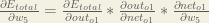
By applying the chain rule we know that:

$\frac{\partial E_{total}}{\partial w_{5}} = \frac{\partial E_{total}}{\partial out_{o1}} * \frac{\partial out_{o1}}{\partial net_{o1}} * \frac{\partial net_{o1}}{\partial w_{5}}$

Visually, here’s what we’re doing:

We need to figure out each piece in this equation.

First, how much does the total error change with respect to the output?

$E_{total} = \frac{1}{2}(target_{o1} - out_{o1})^{2} + \frac{1}{2}(target_{o2} - out_{o2})^{2}$

$\frac{\partial E_{total}}{\partial out_{o1}} = 2 * \frac{1}{2}(target_{o1} - out_{o1})^{2 - 1} * -1 + 0$

$\frac{\partial E_{total}}{\partial out_{o1}} = -(target_{o1} - out_{o1}) = -(0.01 - 0.75136507) = 0.74136507$

$-(target - out)$ is sometimes expressed as $out - target$

When we take the partial derivative of the total error with respect to $out_{o1}$ , the quantity $\frac{1}{2}(target_{o2} - out_{o2})^{2}$ becomes zero because $out_{o1}$ does not affect it which means we’re taking the derivative of a constant which is zero.

Next, how much does the output of $o_1$ change with respect to its total net input?

The partial derivative of the logistic function is the output multiplied by 1 minus the output:

$out_{o1} = \frac{1}{1+e^{-net_{o1}}}$

$\frac{\partial out_{o1}}{\partial net_{o1}} = out_{o1}(1 - out_{o1}) = 0.75136507(1 - 0.75136507) = 0.186815602$

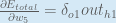
Finally, how much does the total net input of $o1$ change with respect to $w_5$ ?

$net_{o1} = w_5 * out_{h1} + w_6 * out_{h2} + b_2 * 1$

$\frac{\partial net_{o1}}{\partial w_{5}} = 1 * out_{h1} * w_5^{(1 - 1)} + 0 + 0 = out_{h1} = 0.593269992$

Putting it all together:

$\frac{\partial E_{total}}{\partial w_{5}} = \frac{\partial E_{total}}{\partial out_{o1}} * \frac{\partial out_{o1}}{\partial net_{o1}} * \frac{\partial net_{o1}}{\partial w_{5}}$

$\frac{\partial E_{total}}{\partial w_{5}} = 0.74136507 * 0.186815602 * 0.593269992 = 0.082167041$

You’ll often see this calculation combined in the form of the delta rule:

$\frac{\partial E_{total}}{\partial w_{5}} = -(target_{o1} - out_{o1}) * out_{o1}(1 - out_{o1}) * out_{h1}$

Alternatively, we have $\frac{\partial E_{total}}{\partial out_{o1}}$ and $\frac{\partial out_{o1}}{\partial net_{o1}}$ which can be written as $\frac{\partial E_{total}}{\partial net_{o1}}$ , aka $\delta_{o1}$ (the Greek letter delta) aka the node delta. We can use this to rewrite the calculation above:

$\delta_{o1} = \frac{\partial E_{total}}{\partial out_{o1}} * \frac{\partial out_{o1}}{\partial net_{o1}} = \frac{\partial E_{total}}{\partial net_{o1}}$

$\delta_{o1} = -(target_{o1} - out_{o1}) * out_{o1}(1 - out_{o1})$

Therefore:

$\frac{\partial E_{total}}{\partial w_{5}} = \delta_{o1} out_{h1}$

Some sources extract the negative sign from $\delta$ so it would be written as:

$\frac{\partial E_{total}}{\partial w_{5}} = -\delta_{o1} out_{h1}$

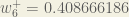
To decrease the error, we then subtract this value from the current weight (optionally multiplied by some learning rate, eta, which we’ll set to 0.5):

$w_5^{+} = w_5 - \eta * \frac{\partial E_{total}}{\partial w_{5}} = 0.4 - 0.5 * 0.082167041 = 0.35891648$

Some sources use $\alpha$ (alpha) to represent the learning rate, others use $\eta$ (eta), and others even use $\epsilon$ (epsilon).

We can repeat this process to get the new weights $w_6$ , $w_7$ , and $w_8$ :

$w_6^{+} = 0.408666186$

$w_7^{+} = 0.511301270$

$w_8^{+} = 0.561370121$

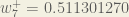
We perform the actual updates in the neural network after we have the new weights leading into the hidden layer neurons (ie, we use the original weights, not the updated weights, when we continue the backpropagation algorithm below).

Hidden Layer

Next, we’ll continue the backwards pass by calculating new values for $w_1$ , $w_2$ , $w_3$ , and $w_4$ .

Big picture, here’s what we need to figure out:

$\frac{\partial E_{total}}{\partial w_{1}} = \frac{\partial E_{total}}{\partial out_{h1}} * \frac{\partial out_{h1}}{\partial net_{h1}} * \frac{\partial net_{h1}}{\partial w_{1}}$

Visually:

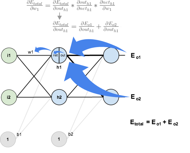
We’re going to use a similar process as we did for the output layer, but slightly different to account for the fact that the output of each hidden layer neuron contributes to the output (and therefore error) of multiple output neurons. We know that $out_{h1}$ affects both $out_{o1}$ and $out_{o2}$ therefore the $\frac{\partial E_{total}}{\partial out_{h1}}$ needs to take into consideration its effect on the both output neurons:

$\frac{\partial E_{total}}{\partial out_{h1}} = \frac{\partial E_{o1}}{\partial out_{h1}} + \frac{\partial E_{o2}}{\partial out_{h1}}$

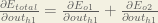
Starting with $\frac{\partial E_{o1}}{\partial out_{h1}}$ :

$\frac{\partial E_{o1}}{\partial out_{h1}} = \frac{\partial E_{o1}}{\partial net_{o1}} * \frac{\partial net_{o1}}{\partial out_{h1}}$

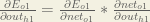
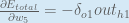
We can calculate $\frac{\partial E_{o1}}{\partial net_{o1}}$ using values we calculated earlier:

$\frac{\partial E_{o1}}{\partial net_{o1}} = \frac{\partial E_{o1}}{\partial out_{o1}} * \frac{\partial out_{o1}}{\partial net_{o1}} = 0.74136507 * 0.186815602 = 0.138498562$

And $\frac{\partial net_{o1}}{\partial out_{h1}}$ is equal to $w_5$ :

$net_{o1} = w_5 * out_{h1} + w_6 * out_{h2} + b_2 * 1$

$\frac{\partial net_{o1}}{\partial out_{h1}} = w_5 = 0.40$

Plugging them in:

$\frac{\partial E_{o1}}{\partial out_{h1}} = \frac{\partial E_{o1}}{\partial net_{o1}} * \frac{\partial net_{o1}}{\partial out_{h1}} = 0.138498562 * 0.40 = 0.055399425$

Following the same process for $\frac{\partial E_{o2}}{\partial out_{h1}}$ , we get:

$\frac{\partial E_{o2}}{\partial out_{h1}} = -0.019049119$

Therefore:

$\frac{\partial E_{total}}{\partial out_{h1}} = \frac{\partial E_{o1}}{\partial out_{h1}} + \frac{\partial E_{o2}}{\partial out_{h1}} = 0.055399425 + -0.019049119 = 0.036350306$

Now that we have $\frac{\partial E_{total}}{\partial out_{h1}}$ , we need to figure out $\frac{\partial out_{h1}}{\partial net_{h1}}$ and then $\frac{\partial net_{h1}}{\partial w}$ for each weight:

$out_{h1} = \frac{1}{1+e^{-net_{h1}}}$

$\frac{\partial out_{h1}}{\partial net_{h1}} = out_{h1}(1 - out_{h1}) = 0.59326999(1 - 0.59326999 ) = 0.241300709$

We calculate the partial derivative of the total net input to $h_1$ with respect to $w_1$ the same as we did for the output neuron:

$net_{h1} = w_1 * i_1 + w_3 * i_2 + b_1 * 1$

$\frac{\partial net_{h1}}{\partial w_1} = i_1 = 0.05$

Putting it all together:

$\frac{\partial E_{total}}{\partial w_{1}} = \frac{\partial E_{total}}{\partial out_{h1}} * \frac{\partial out_{h1}}{\partial net_{h1}} * \frac{\partial net_{h1}}{\partial w_{1}}$

$\frac{\partial E_{total}}{\partial w_{1}} = 0.036350306 * 0.241300709 * 0.05 = 0.000438568$

You might also see this written as:

$\frac{\partial E_{total}}{\partial w_{1}} = (\sum\limits_{o}{\frac{\partial E_{total}}{\partial out_{o}} * \frac{\partial out_{o}}{\partial net_{o}} * \frac{\partial net_{o}}{\partial out_{h1}}}) * \frac{\partial out_{h1}}{\partial net_{h1}} * \frac{\partial net_{h1}}{\partial w_{1}}$

$\frac{\partial E_{total}}{\partial w_{1}} = (\sum\limits_{o}{\delta_{o} * w_{ho}}) * out_{h1}(1 - out_{h1}) * i_{1}$

$\frac{\partial E_{total}}{\partial w_{1}} = \delta_{h1}i_{1}$

We can now update $w_1$ :

$w_1^{+} = w_1 - \eta * \frac{\partial E_{total}}{\partial w_{1}} = 0.15 - 0.5 * 0.000438568 = 0.149780716$

Repeating this for $w_2$ , $w_3$ , and $w_4$

$w_2^{+} = 0.19956143$

$w_3^{+} = 0.24975114$

$w_4^{+} = 0.29950229$

Finally, we’ve updated all of our weights! When we fed forward the 0.05 and 0.1 inputs originally, the error on the network was 0.298371109. After this first round of backpropagation, the total error is now down to 0.291027924. It might not seem like much, but after repeating this process 10,000 times, for example, the error plummets to 0.0000351085. At this point, when we feed forward 0.05 and 0.1, the two outputs neurons generate 0.015912196 (vs 0.01 target) and 0.984065734 (vs 0.99 target).

If you’ve made it this far and found any errors in any of the above or can think of any ways to make it clearer for future readers, don’t hesitate to drop me a note. Thanks!

And while I have you…

Again, if you liked this tutorial, please check out Emergent Mind, a site I’m building with an end goal of explaining AI/ML concepts in a similar style as this post. Feedback very much welcome!

1,090 thoughts on “A Step by Step Backpropagation Example”

Pingback: I’m going to write more often. For real this time. – Matt Mazur
Hugo Wainwright (@_frugs) says:

November 26, 2015 at 4:01 pm

Having the numbers and the calculations here has really helped me in debugging my implementation of this, so a big thanks for that!

I notice you’ve missed out the calculations for the updates of the bias; I realise that it’s fairly trivial to work out dneto1/db and dneth1/db and chain rule them to find out dEtotal/db, but is this intentional?

Reply
1. Mazur says:
  
  November 28, 2015 at 3:36 pm
  
  Hey Hugo, it’s simple because the materials I read did not include updating the bias :).
  
  Does updating the bias have a big impact on the training efficiency?
  
  Reply
Constantine says:

December 1, 2015 at 6:27 am

Man, you’re awesome! Thank you so much for the post! I wish I’d found it 10 days ago.

There’s one thing I don’t understand — when you’re updating the weight, why’re you *substracting* the derivative? I’ve read another paper, and there the author does *addition* instead. On what does it depends?

Reply
lsatish says:

December 1, 2015 at 9:46 am

Elegantly explained. Thanks for writing.

Reply
Constantine says:

December 2, 2015 at 5:13 am

Just to let you know — here seems to be a bug. It is that the comments here are invisible unless one leave a comment themselves. And after that, a day later, comments again disappears. I don’t see a button like «Show comments», so it is definitely a bug.

Reply
deepak says:

December 2, 2015 at 12:39 pm

thanks for the simple explanation

Reply
Aledee says:

December 4, 2015 at 12:26 pm

Why are network outputs set to 0.01 and 0.99? Why are they not set to 0 and 1? In most texts I see them as 0 and 1.

Reply
tannerbohn says:

December 6, 2015 at 4:18 am

Did you skip the bias update calculations?

Reply
1. tannerbohn says:
  
  December 6, 2015 at 4:23 am
  
  never mind! Just saw the other comments!
  
  Reply
gareththegeek says:

December 7, 2015 at 8:21 am

Thanks for the detailed tutorial. It has been really useful in implementing this algorithm in C#! One discrepancy, when I run this example through my code, I get a different value for one of the hidden layer differentials:

\frac{\partial E_{o2}}{\partial out_{h1}} = -0.019049119

I make this -0.017144205

Which of us is correct?

Reply
1. gareththegeek says:
  
  December 8, 2015 at 3:55 am
  
  Nevermind! I found my mistake.
  Thanks again for the informative article.
  
  Reply
Mostafa Razavi says:

December 7, 2015 at 1:09 pm

That was heaven, thanks a million.

Reply
Sonal Shrivastava says:

December 8, 2015 at 11:40 am

That was awesome. Thank a ton.

Reply
Nayantara says:

December 9, 2015 at 7:29 am

Hi Matt, Can you also please provide a similar example for a convolutional neural network which uses at least 1 convolutional layer and 1 pooling layer ? Surprisingly, I haven’t been able to find ANY similar example for backpropagation, on the internet, for Conv. Neural Network.
TIA.

Reply
1. Mazur says:
  
  December 9, 2015 at 8:36 am
  
  I haven’t learnt that yet. If you find a good tutorial please let me know.
  
  Reply
Pingback: A Step by Step Backpropagation Example | Matt Mazur | tensorflowgraphs
payamrastogi says:

December 11, 2015 at 4:24 am

All hail to “The” Mazur

Reply
Pingback: The State of Emergent Mind – Matt Mazur
Louis Hong says:

December 11, 2015 at 4:41 pm

Thank you so much for your most comprehensive tutorial ever on the internet.

Reply
ad says:

December 17, 2015 at 1:49 am

why is bias not updated ?

Reply
1. Mazur says:
  
  December 17, 2015 at 9:23 am
  
  Hey, in the tutorials I went through they didn’t update the bias which is why I didn’t include it here.
  
  Reply
  1. justaguy says:
    
    December 24, 2015 at 8:54 pm
    
    Typically, bias error is equal to the sum of the errors of the neurons that the bias connects to. For example, in regards to your example, b1_error = h1_error + h2_error. Updating the bias’ weight would be adding the product of the summed errors and the learning rate to the bias, ex. b1_weight = b1_error * learning_rate. Although many problems can be learned by a neural network without adjusting biases and there may be better ways to adust bias weights. Also, updating bias weights may cause problems with learning as opposed to keeping them static. As usual with neural networks, through experimentation you may discover more optimal designs.
    
    Reply
    1. patriczhao says:
      
      January 13, 2016 at 1:30 am
      
      nice explanations, thanks.
      
      Reply
Ahad Khan says:

December 20, 2015 at 2:26 am

This is perfect. I am able to visualize back propagation algo better after reading this article. Thanks once again!

Reply
sunlyt says:

December 21, 2015 at 12:57 am

Brilliant. Thank-you!

Reply
garky says:

December 24, 2015 at 8:25 am

If we have more than one sample in our dataset how we can train it by considering all samples, not just one sample?

Reply
Daniel Zukowski says:

December 24, 2015 at 2:32 pm

Invaluable resource you’ve produced. Thank you for this clear, comprehensive, visual explanation. The inner mechanics of backpropagation are no longer a mystery to me.

Reply
Long Pham says:

December 26, 2015 at 10:58 am

precisely, intuitively, very easy to understand, great work, thank you.

Reply
Dionisius AN says:

December 27, 2015 at 1:16 pm

Thank you very much ,it’s help me well, u really give detail direction to allow me imagine how it works. I really appreciate it. May God repay your kindness thousand time than u do.

Reply
singhrocks91 says:

December 28, 2015 at 1:35 am

Thank You. I have a better insight now

Reply
DGelling says:

January 1, 2016 at 6:48 pm

Shouldn’t the derivative of out_o1 wrt net_o1 be net_o1*(1-net_o1)?

Reply
1. NaanTadow says:
  
  February 24, 2016 at 1:10 am
  
  No the one stated above is correct, see here for the steps on the gradient of the activation function with respect to its input value (net): https://theclevermachine.wordpress.com/2014/09/08/derivation-derivatives-for-common-neural-network-activation-functions/
  
  Oh and thanks for this Matt – was able to work through your breakdown of the partial derivatives for the Andrew Ng ML Course on coursera :D
  
  Reply
dreugeworst says:

January 1, 2016 at 6:55 pm

shoudn’t the derivative of out_o1 wrt net_o1 be net_o1(1-net_o1)?

Reply
Pingback: Coding Neural networks | Bits and pieces
Pingback: Apprendre à coder un réseau de neurones | Actuaires – Big Data
Pingback: Contextual Integration Is the Secret Weapon of Predictive Analytics
Aro says:

January 10, 2016 at 6:23 pm

thanks so much, I haven’t see tutorial before like this.

Reply
Derive Me says:

January 12, 2016 at 1:22 am

Hello. I don’t understand, below the phrase “First, how much does the total error change with respect to the output?”, why there is a (*-1) in the second equation, that eventually changes the result to -(target – output) instead of just (target – output). Can you help me understand?

Thank you!

Reply
1. Flipperty says:
  
  March 25, 2016 at 2:40 pm
  
  I’d love to see an answer to this as well: where does that -1 come from? I can make it come from the derivation using the power rule. Help!
  
  Reply
  1. Robert Lee says:
    
    June 4, 2017 at 5:54 am
    
    Same here, not quite understand where the -1 come from.
    
    Reply
angie1pecht says:

January 17, 2016 at 8:52 pm

This helped me a lot. Thank you so much!

Reply
LEarning AI again says:

January 18, 2016 at 4:26 pm

This was awesome. Thanks so much!

Reply
Ashish says:

January 19, 2016 at 7:21 am

Thanks a lot Matt… Appreciated the effort, Kudos

Reply
Pingback: Learning How To Code Neural Networks | ipythonblog
Tariq says:

January 20, 2016 at 12:03 pm

If the error is “squared” but simply E = sum (target – output) , you can still do the calculus to work out the error gradient .. and then update the weights. Where did I go wrong with this logic?

Reply
Elliot says:

January 28, 2016 at 9:03 am

Good afternoon, dear Matt Mazur!

Thank you very much for writing so complete and comprehensive tutorial, everything is understandable and written in accessible way! If is it posdible may I ask following question if I need to compute Jacobian Matrix elements in formula for computing Error Gradient with respect to weight dEtotal/dwi I should just percieve Etotal not as the full error from all outputs but as an error from some certain single output, could you please say is this correct? Could you please say are you not planning to make a simillar tutorial but for computing second order derivatives (backpropagation with partial derivatives of second order)? I have searching internet for tutorial of calculating second order derivatives in backpropagation but did not found anything. Maybe you know some good tutorials for it? I have know that second order partial derivatives (elements of Hessian Matrix) can be approximated by multiplaying Jacobians but wanted to find it’s exact non approximated calculation. Thank you in advance for your reply!

Sincerely

Reply
Kumaresan Kaliappan says:

January 30, 2016 at 12:31 am

Hi Really it is a great tutorial

Reply
Pulley says:

February 1, 2016 at 9:52 pm

hello Matt, Can you please tell me that after updating all weights in first iteration I should update the values of all ‘h’ at-last in first iteration or not.

Reply
Tariq says:

February 3, 2016 at 5:00 pm

Why is the error assumed to be sum squared? The errors are not Gaussian. In fact you don’t even sum over the output nodes when updating weights – you do it per node, so there is no need to ensure the sum is >0. Here’s my challenge… http://makeyourownneuralnetwork.blogspot.co.uk/2016/01/why-squared-error-cost-function.html

Reply
Behroz Ahmad Ali says:

February 6, 2016 at 8:01 am

Thank you for such a comprehensive explanation of backpropagation. I have been trying to understand backpropagation for months but today I finally understood it after reading your this post.

Reply
1. Tariq says:
  
  February 8, 2016 at 10:57 am
  
  i am writing a gentle intro to neural networks – aimed at being accessible to someone at school approx age 15… here is a draft which includes a very very gentle intro to backprop
  
  https://goo.gl/7uxHlm
  
  i’d appreciate feedback to @myoneuralnet
  
  Reply
Rebeka Sultana says:

February 16, 2016 at 12:59 am

Thank you so much.

Reply
Ron says:

February 21, 2016 at 1:10 pm

Firstly, thank you VERY much for a great walkthrough of all the steps involved with real values. I managed to create a quick implementation of the methods used, and was able to train successfully.

I was looking to use this setup (but with 4 inputs / 3 outputs) for the famous iris data (http://archive.ics.uci.edu/ml/datasets/Iris). The 3 outputs would be 0.0-1.0 for each classification, as there would be an output weight towards each type.

Unfortunately it doesn’t seem to be able to resolve to an always low error value, and fluctuates drastically as it trains. Is this an indication that a second layer is needed for this type of data?

Reply
Werner says:

February 22, 2016 at 5:44 am

The first explanation I read that actually makes sense to me. Most just seem to start shovelling maths in your face in the name of “not making it simpler that they should”. Now let’s hope my AI will finally be able to play a game of draughts.

Reply
admin says:

February 22, 2016 at 9:20 am

It helps me a lot. thanks for the work!!!

Reply
Name(required) says:

February 24, 2016 at 8:55 pm

Thanks great tutorial. By any chance would you know how to train for 2 hidden layers?

Reply
Name(required) says:

February 24, 2016 at 9:04 pm

Great tutorial. By any chance do you know how do backpropagate 2 hidden layers?

Reply
1. Mazur says:
  
  February 25, 2016 at 8:22 am
  
  I do not, sorry.
  
  Reply
Kiran says:

February 25, 2016 at 12:29 am

Thank you so much! The explanation was so intuitive.

Reply
Anon says:

February 25, 2016 at 11:18 pm

Thank you! The way you explain this is very intuitive.

Reply
tariq says:

February 26, 2016 at 9:38 am

I’d love your feedback on my attempt to explain the maths and ideas underlying neuralnetworks and backrpop.

Here’s an early draft online. The aim for me is to reach as many people as possible inck teenagers with school maths.

http://makeyourownneuralnetwork.blogspot.co.uk/2016/02/early-draft-feedback-wanted.html

Reply
1. Garett Ridge AndThenSomeMoreWords says:
  
  March 1, 2016 at 5:45 pm
  
  I have a presentation tomorrow on neural networks in a grad class that I’m drowning in. This book is going to save my life
  
  Reply