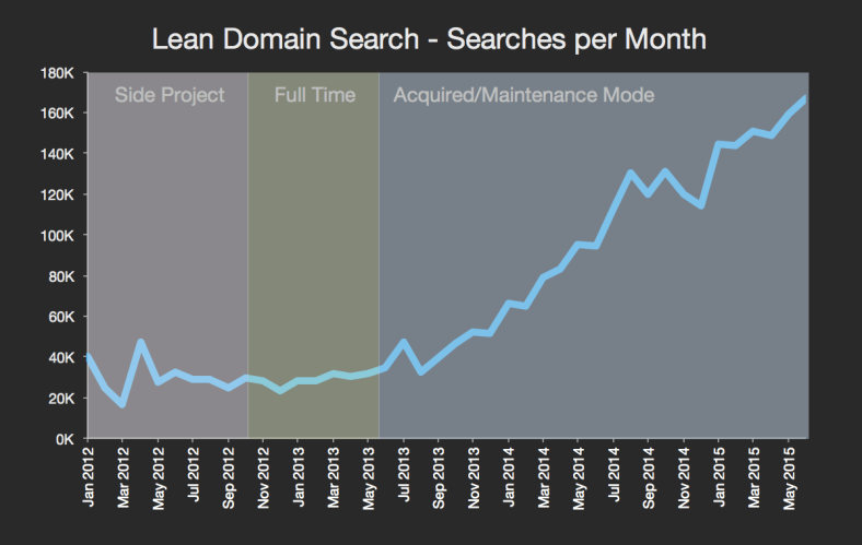
Lean Domain Search, despite almost no work since its acquisition by Automattic two years ago, has continued to thrive, now handling more than 160,000 searches per month:
It’s monthly growth rate works out to be about 6.5%. Not huge, but not bad for maintenance mode. :)
A few years ago I wrote about a bot I built in high school to play an online multiplayer Tetris game called TetriNET. The tl;dr is that I got into TetriNET with some friends, built a bot to automate the play, and eventually entered my school’s science fair with it and wound up making it to internationals. As you can imagine, I was pretty cool in high school…
Anyway, when I wrote the post Github was just getting off the ground and it didn’t even occur to me at the time to open source the code there; instead I just zipped up the Visual Basic Project (go VB6!) and linked to it from the post.
Happily, I have gained a little bit more experience with Git and Github since then so I took some to clean up the code (converting CRLF line endings to LF, spaces to tabs, etc) and finally published it.
Backpropagation is a common method for training a neural network. There is no shortage of papers online that attempt to explain how backpropagation works, but few that include an example with actual numbers. This post is my attempt to explain how it works with a concrete example that folks can compare their own calculations to in order to ensure they understand backpropagation correctly.
Backpropagation in Python
You can play around with a Python script that I wrote that implements the backpropagation algorithm in this Github repo.
Continue learning with Emergent Mind
If you find this tutorial useful and want to continue learning about AI/ML, I encourage you to check out Emergent Mind, a new website I’m working on that uses GPT-4 to surface and explain cutting-edge AI/ML papers:
In time, I hope to use AI to explain complex AI/ML topics on Emergent Mind in a style similar to what you’ll find in the tutorial below.
Now, on with the backpropagation tutorial…
Overview
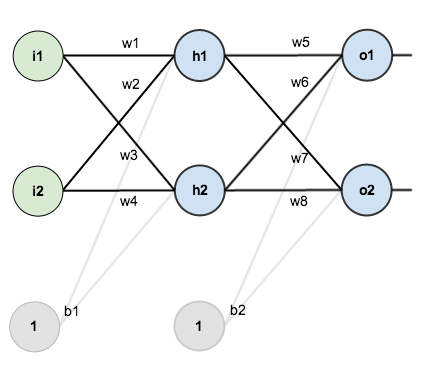
For this tutorial, we’re going to use a neural network with two inputs, two hidden neurons, two output neurons. Additionally, the hidden and output neurons will include a bias.
Here’s the basic structure:
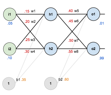
In order to have some numbers to work with, here are the initial weights, the biases, and training inputs/outputs:
The goal of backpropagation is to optimize the weights so that the neural network can learn how to correctly map arbitrary inputs to outputs.
For the rest of this tutorial we’re going to work with a single training set: given inputs 0.05 and 0.10, we want the neural network to output 0.01 and 0.99.
The Forward Pass
To begin, lets see what the neural network currently predicts given the weights and biases above and inputs of 0.05 and 0.10. To do this we’ll feed those inputs forward though the network.
We figure out the total net input to each hidden layer neuron, squash the total net input using an activation function (here we use the logistic function), then repeat the process with the output layer neurons.
Total net input is also referred to as just net input by some sources.
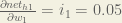
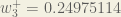
Here’s how we calculate the total net input for :
We then squash it using the logistic function to get the output of :
Carrying out the same process for we get:
We repeat this process for the output layer neurons, using the output from the hidden layer neurons as inputs.
Here’s the output for :
And carrying out the same process for we get:
Calculating the Total Error
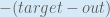
We can now calculate the error for each output neuron using the squared error function and sum them to get the total error:
Some sources refer to the target as the ideal and the output as the actual.
The is included so that exponent is cancelled when we differentiate later on. The result is eventually multiplied by a learning rate anyway so it doesn’t matter that we introduce a constant here [1].
For example, the target output for is 0.01 but the neural network output 0.75136507, therefore its error is:
Repeating this process for (remembering that the target is 0.99) we get:
The total error for the neural network is the sum of these errors:
The Backwards Pass
Our goal with backpropagation is to update each of the weights in the network so that they cause the actual output to be closer the target output, thereby minimizing the error for each output neuron and the network as a whole.
Output Layer
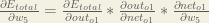
Consider . We want to know how much a change in affects the total error, aka .
is read as “the partial derivative of with respect to “. You can also say “the gradient with respect to ”.
We need to figure out each piece in this equation.
First, how much does the total error change with respect to the output?
is sometimes expressed as
When we take the partial derivative of the total error with respect to , the quantity becomes zero because does not affect it which means we’re taking the derivative of a constant which is zero.
Next, how much does the output of change with respect to its total net input?
Finally, how much does the total net input of change with respect to ?
Putting it all together:
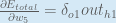
You’ll often see this calculation combined in the form of the delta rule:
Alternatively, we have and which can be written as , aka (the Greek letter delta) aka the node delta. We can use this to rewrite the calculation above:
Therefore:
Some sources extract the negative sign from so it would be written as:
To decrease the error, we then subtract this value from the current weight (optionally multiplied by some learning rate, eta, which we’ll set to 0.5):
We can repeat this process to get the new weights , , and :
We perform the actual updates in the neural network after we have the new weights leading into the hidden layer neurons (ie, we use the original weights, not the updated weights, when we continue the backpropagation algorithm below).
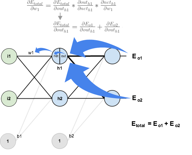
Hidden Layer
Next, we’ll continue the backwards pass by calculating new values for , , , and .
Big picture, here’s what we need to figure out:
Visually:
We’re going to use a similar process as we did for the output layer, but slightly different to account for the fact that the output of each hidden layer neuron contributes to the output (and therefore error) of multiple output neurons. We know that affects both and therefore the needs to take into consideration its effect on the both output neurons:
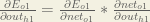
Starting with :
We can calculate using values we calculated earlier:
And is equal to :
Plugging them in:
Following the same process for , we get:
Therefore:
Now that we have , we need to figure out and then for each weight:
We calculate the partial derivative of the total net input to with respect to the same as we did for the output neuron:
Putting it all together:
You might also see this written as:
We can now update :
Repeating this for , , and
Finally, we’ve updated all of our weights! When we fed forward the 0.05 and 0.1 inputs originally, the error on the network was 0.298371109. After this first round of backpropagation, the total error is now down to 0.291027924. It might not seem like much, but after repeating this process 10,000 times, for example, the error plummets to 0.0000351085. At this point, when we feed forward 0.05 and 0.1, the two outputs neurons generate 0.015912196 (vs 0.01 target) and 0.984065734 (vs 0.99 target).
If you’ve made it this far and found any errors in any of the above or can think of any ways to make it clearer for future readers, don’t hesitate to drop me a note. Thanks!
And while I have you…
Again, if you liked this tutorial, please check out Emergent Mind, a site I’m building with an end goal of explaining AI/ML concepts in a similar style as this post. Feedback very much welcome!
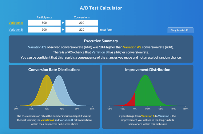
I spent some time recently working on a small side project that I’m excited to share with you all today. It’s an A/B test significance calculator and you can check it out at ABTestCalculator.com.
What’s an A/B test significance calculator, you ask? At a high level, A/B testing is a technique that allows you to improve your website by showing visitors one of several versions of something and then measuring the impact each version has on some other event. For example, you might A/B test the wording of a button on your homepage and find that it increases the number of people who sign up by 10%. An A/B test significance calculator helps you analyze the results of an A/B test to determine whether there is a statistically significant change that is not just the result of random chance.
Why build another? Three reasons: to learn the math, to get better at JavaScript, and to build a tool that makes the results of an A/B test easier to understand.
I think most of these other tools do users a disservice by not clearly explaining how to interpret the results. They tend to throw around the percentage improvement and significance figures without explaining what they mean which in the past has led me to make uninformed and often wrong decisions. Worse, most don’t tell you when you don’t have enough participants or conversions in your test and will happily apply statistical analysis to your results even when those methods don’t apply.
It is my hope with this tool that users leave with a clearer understand of how to interpret the results. A few features:
An executive summary that provides an overview in plain English about how to interpret the results
One graph showing where the true conversion rate for each variation falls (using something called a Wald approximation) and another showing the percentage change between those two distributions
It handles ties as well as tests where there aren’t enough participants or conversions to come to a conclusion
Results are significant when there is at least a 90% chance that one variation will lead to an improvement
The ability to copy a URL for the results to make them easier to share
If you have any suggestions on how to make it better please don’t hesitate to let me know.
On the coding site of things, most of the JavaScript I’ve done in the past (including Preceden and Lean Domain Search) has been with lots and lots of messy jQuery. A lot of new JavaScript technologies have come out in the last few years and I was put on a project at Automattic not too long ago that uses many of them. I fumbled around with it, getting stuff done but not really understanding the fundamentals.
I’m happy to say that this tool uses React for the view layer, NPM and Browserify for dependency management, Gulp for its build system, parts of ES6 for the code (courtesy of Babel), JSHint for code analysis, Mocha for testing, and Github Pages for hosting — all of which I had little to no experience with when I started this project. If you’re interested in checking it out, all of the code is open source (my first!) so you can view it on Github.
This project is the best JavaScript I know how to do so if you do check out the code, please let me know if you have any suggestions on how to improve it.
One last note in case you were wondering about the domain: the former owner had a simple A/B test calculator up on it, but wasn’t actively working on it so I found his email via WHOIS, offered him $200 for it, he countered with $700, I countered with $300 and we had a deal. Normally I wouldn’t pay someone for a domain (I heard there is this amazing service to help people find available domains…), but the price was right and I figured it was worth it for the credibility and SEO value it adds. When I showed him the new site recently all he responded with was “I’m pretty glad I sold the domain now!” which was nice :).


 :
:


 we get:
 :
:


 we get:

 is included so that exponent is cancelled when we differentiate later on. The result is eventually multiplied by a learning rate anyway so it doesn’t matter that we introduce a constant here [
 (remembering that the target is 0.99) we get:

 . We want to know how much a change in
  .
. is read as “the partial derivative of
  with respect to
  “. You can also say “the gradient with respect to


 is sometimes expressed as
 , the quantity
  becomes zero because
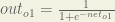

 change with respect to


 and
and  which can be written as
  , aka
, aka  (the Greek letter delta) aka the node delta. We can use this to rewrite the calculation above:

 so it would be written as:

 (alpha) to represent the learning rate,
  (eta), and
  (epsilon).
 ,
,  , and
, and  :
:
 ,
,  ,
,  , and
, and  .
.
 affects both
  and
and  therefore the
  needs to take into consideration its effect on the both output neurons:
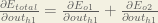
 :
:
 using values we calculated earlier:
 is equal to

 , we get:
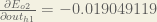

 and then
  for each weight: