A Step by Step Backpropagation Example

March 17, 2015February 23, 2024Mazur

Background

Backpropagation is a common method for training a neural network. There is no shortage of papers online that attempt to explain how backpropagation works, but few that include an example with actual numbers. This post is my attempt to explain how it works with a concrete example that folks can compare their own calculations to in order to ensure they understand backpropagation correctly.

Backpropagation in Python

You can play around with a Python script that I wrote that implements the backpropagation algorithm in this Github repo.

Continue learning with Emergent Mind

If you find this tutorial useful and want to continue learning about AI/ML, I encourage you to check out Emergent Mind, a new website I’m working on that uses GPT-4 to surface and explain cutting-edge AI/ML papers:

In time, I hope to use AI to explain complex AI/ML topics on Emergent Mind in a style similar to what you’ll find in the tutorial below.

Now, on with the backpropagation tutorial…

Overview

For this tutorial, we’re going to use a neural network with two inputs, two hidden neurons, two output neurons. Additionally, the hidden and output neurons will include a bias.

Here’s the basic structure:

In order to have some numbers to work with, here are the initial weights, the biases, and training inputs/outputs:

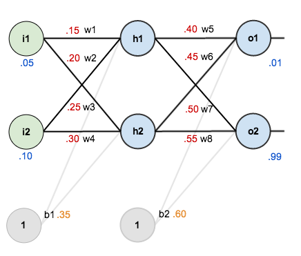
The goal of backpropagation is to optimize the weights so that the neural network can learn how to correctly map arbitrary inputs to outputs.

For the rest of this tutorial we’re going to work with a single training set: given inputs 0.05 and 0.10, we want the neural network to output 0.01 and 0.99.

The Forward Pass

To begin, lets see what the neural network currently predicts given the weights and biases above and inputs of 0.05 and 0.10. To do this we’ll feed those inputs forward though the network.

We figure out the total net input to each hidden layer neuron, squash the total net input using an activation function (here we use the logistic function), then repeat the process with the output layer neurons.

Total net input is also referred to as just net input by some sources.

Here’s how we calculate the total net input for $h_1$ :

$net_{h1} = w_1 * i_1 + w_2 * i_2 + b_1 * 1$

$net_{h1} = 0.15 * 0.05 + 0.2 * 0.1 + 0.35 * 1 = 0.3775$

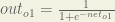
We then squash it using the logistic function to get the output of $h_1$ :

$out_{h1} = \frac{1}{1+e^{-net_{h1}}} = \frac{1}{1+e^{-0.3775}} = 0.593269992$

Carrying out the same process for $h_2$ we get:

$out_{h2} = 0.596884378$

We repeat this process for the output layer neurons, using the output from the hidden layer neurons as inputs.

Here’s the output for $o_1$ :

$net_{o1} = w_5 * out_{h1} + w_6 * out_{h2} + b_2 * 1$

$net_{o1} = 0.4 * 0.593269992 + 0.45 * 0.596884378 + 0.6 * 1 = 1.105905967$

$out_{o1} = \frac{1}{1+e^{-net_{o1}}} = \frac{1}{1+e^{-1.105905967}} = 0.75136507$

And carrying out the same process for $o_2$ we get:

$out_{o2} = 0.772928465$

Calculating the Total Error

We can now calculate the error for each output neuron using the squared error function and sum them to get the total error:

$E_{total} = \sum \frac{1}{2}(target - output)^{2}$

Some sources refer to the target as the ideal and the output as the actual.

The $\frac{1}{2}$ is included so that exponent is cancelled when we differentiate later on. The result is eventually multiplied by a learning rate anyway so it doesn’t matter that we introduce a constant here [1].

For example, the target output for $o_1$ is 0.01 but the neural network output 0.75136507, therefore its error is:

$E_{o1} = \frac{1}{2}(target_{o1} - out_{o1})^{2} = \frac{1}{2}(0.01 - 0.75136507)^{2} = 0.274811083$

Repeating this process for $o_2$ (remembering that the target is 0.99) we get:

$E_{o2} = 0.023560026$

The total error for the neural network is the sum of these errors:

$E_{total} = E_{o1} + E_{o2} = 0.274811083 + 0.023560026 = 0.298371109$

The Backwards Pass

Our goal with backpropagation is to update each of the weights in the network so that they cause the actual output to be closer the target output, thereby minimizing the error for each output neuron and the network as a whole.

Output Layer

Consider $w_5$ . We want to know how much a change in $w_5$ affects the total error, aka $\frac{\partial E_{total}}{\partial w_{5}}$ .

$\frac{\partial E_{total}}{\partial w_{5}}$ is read as “the partial derivative of $E_{total}$ with respect to $w_{5}$ “. You can also say “the gradient with respect to $w_{5}$ ”.

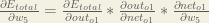
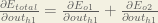
By applying the chain rule we know that:

$\frac{\partial E_{total}}{\partial w_{5}} = \frac{\partial E_{total}}{\partial out_{o1}} * \frac{\partial out_{o1}}{\partial net_{o1}} * \frac{\partial net_{o1}}{\partial w_{5}}$

Visually, here’s what we’re doing:

We need to figure out each piece in this equation.

First, how much does the total error change with respect to the output?

$E_{total} = \frac{1}{2}(target_{o1} - out_{o1})^{2} + \frac{1}{2}(target_{o2} - out_{o2})^{2}$

$\frac{\partial E_{total}}{\partial out_{o1}} = 2 * \frac{1}{2}(target_{o1} - out_{o1})^{2 - 1} * -1 + 0$

$\frac{\partial E_{total}}{\partial out_{o1}} = -(target_{o1} - out_{o1}) = -(0.01 - 0.75136507) = 0.74136507$

$-(target - out)$ is sometimes expressed as $out - target$

When we take the partial derivative of the total error with respect to $out_{o1}$ , the quantity $\frac{1}{2}(target_{o2} - out_{o2})^{2}$ becomes zero because $out_{o1}$ does not affect it which means we’re taking the derivative of a constant which is zero.

Next, how much does the output of $o_1$ change with respect to its total net input?

The partial derivative of the logistic function is the output multiplied by 1 minus the output:

$out_{o1} = \frac{1}{1+e^{-net_{o1}}}$

$\frac{\partial out_{o1}}{\partial net_{o1}} = out_{o1}(1 - out_{o1}) = 0.75136507(1 - 0.75136507) = 0.186815602$

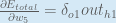
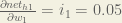
Finally, how much does the total net input of $o1$ change with respect to $w_5$ ?

$net_{o1} = w_5 * out_{h1} + w_6 * out_{h2} + b_2 * 1$

$\frac{\partial net_{o1}}{\partial w_{5}} = 1 * out_{h1} * w_5^{(1 - 1)} + 0 + 0 = out_{h1} = 0.593269992$

Putting it all together:

$\frac{\partial E_{total}}{\partial w_{5}} = \frac{\partial E_{total}}{\partial out_{o1}} * \frac{\partial out_{o1}}{\partial net_{o1}} * \frac{\partial net_{o1}}{\partial w_{5}}$

$\frac{\partial E_{total}}{\partial w_{5}} = 0.74136507 * 0.186815602 * 0.593269992 = 0.082167041$

You’ll often see this calculation combined in the form of the delta rule:

$\frac{\partial E_{total}}{\partial w_{5}} = -(target_{o1} - out_{o1}) * out_{o1}(1 - out_{o1}) * out_{h1}$

Alternatively, we have $\frac{\partial E_{total}}{\partial out_{o1}}$ and $\frac{\partial out_{o1}}{\partial net_{o1}}$ which can be written as $\frac{\partial E_{total}}{\partial net_{o1}}$ , aka $\delta_{o1}$ (the Greek letter delta) aka the node delta. We can use this to rewrite the calculation above:

$\delta_{o1} = \frac{\partial E_{total}}{\partial out_{o1}} * \frac{\partial out_{o1}}{\partial net_{o1}} = \frac{\partial E_{total}}{\partial net_{o1}}$

$\delta_{o1} = -(target_{o1} - out_{o1}) * out_{o1}(1 - out_{o1})$

Therefore:

$\frac{\partial E_{total}}{\partial w_{5}} = \delta_{o1} out_{h1}$

Some sources extract the negative sign from $\delta$ so it would be written as:

$\frac{\partial E_{total}}{\partial w_{5}} = -\delta_{o1} out_{h1}$

To decrease the error, we then subtract this value from the current weight (optionally multiplied by some learning rate, eta, which we’ll set to 0.5):

$w_5^{+} = w_5 - \eta * \frac{\partial E_{total}}{\partial w_{5}} = 0.4 - 0.5 * 0.082167041 = 0.35891648$

Some sources use $\alpha$ (alpha) to represent the learning rate, others use $\eta$ (eta), and others even use $\epsilon$ (epsilon).

We can repeat this process to get the new weights $w_6$ , $w_7$ , and $w_8$ :

$w_6^{+} = 0.408666186$

$w_7^{+} = 0.511301270$

$w_8^{+} = 0.561370121$

We perform the actual updates in the neural network after we have the new weights leading into the hidden layer neurons (ie, we use the original weights, not the updated weights, when we continue the backpropagation algorithm below).

Hidden Layer

Next, we’ll continue the backwards pass by calculating new values for $w_1$ , $w_2$ , $w_3$ , and $w_4$ .

Big picture, here’s what we need to figure out:

$\frac{\partial E_{total}}{\partial w_{1}} = \frac{\partial E_{total}}{\partial out_{h1}} * \frac{\partial out_{h1}}{\partial net_{h1}} * \frac{\partial net_{h1}}{\partial w_{1}}$

Visually:

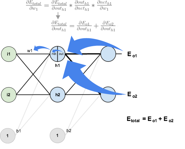
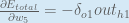
We’re going to use a similar process as we did for the output layer, but slightly different to account for the fact that the output of each hidden layer neuron contributes to the output (and therefore error) of multiple output neurons. We know that $out_{h1}$ affects both $out_{o1}$ and $out_{o2}$ therefore the $\frac{\partial E_{total}}{\partial out_{h1}}$ needs to take into consideration its effect on the both output neurons:

$\frac{\partial E_{total}}{\partial out_{h1}} = \frac{\partial E_{o1}}{\partial out_{h1}} + \frac{\partial E_{o2}}{\partial out_{h1}}$

Starting with $\frac{\partial E_{o1}}{\partial out_{h1}}$ :

$\frac{\partial E_{o1}}{\partial out_{h1}} = \frac{\partial E_{o1}}{\partial net_{o1}} * \frac{\partial net_{o1}}{\partial out_{h1}}$

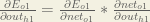
We can calculate $\frac{\partial E_{o1}}{\partial net_{o1}}$ using values we calculated earlier:

$\frac{\partial E_{o1}}{\partial net_{o1}} = \frac{\partial E_{o1}}{\partial out_{o1}} * \frac{\partial out_{o1}}{\partial net_{o1}} = 0.74136507 * 0.186815602 = 0.138498562$

And $\frac{\partial net_{o1}}{\partial out_{h1}}$ is equal to $w_5$ :

$net_{o1} = w_5 * out_{h1} + w_6 * out_{h2} + b_2 * 1$

$\frac{\partial net_{o1}}{\partial out_{h1}} = w_5 = 0.40$

Plugging them in:

$\frac{\partial E_{o1}}{\partial out_{h1}} = \frac{\partial E_{o1}}{\partial net_{o1}} * \frac{\partial net_{o1}}{\partial out_{h1}} = 0.138498562 * 0.40 = 0.055399425$

Following the same process for $\frac{\partial E_{o2}}{\partial out_{h1}}$ , we get:

$\frac{\partial E_{o2}}{\partial out_{h1}} = -0.019049119$

Therefore:

$\frac{\partial E_{total}}{\partial out_{h1}} = \frac{\partial E_{o1}}{\partial out_{h1}} + \frac{\partial E_{o2}}{\partial out_{h1}} = 0.055399425 + -0.019049119 = 0.036350306$

Now that we have $\frac{\partial E_{total}}{\partial out_{h1}}$ , we need to figure out $\frac{\partial out_{h1}}{\partial net_{h1}}$ and then $\frac{\partial net_{h1}}{\partial w}$ for each weight:

$out_{h1} = \frac{1}{1+e^{-net_{h1}}}$

$\frac{\partial out_{h1}}{\partial net_{h1}} = out_{h1}(1 - out_{h1}) = 0.59326999(1 - 0.59326999 ) = 0.241300709$

We calculate the partial derivative of the total net input to $h_1$ with respect to $w_1$ the same as we did for the output neuron:

$net_{h1} = w_1 * i_1 + w_3 * i_2 + b_1 * 1$

$\frac{\partial net_{h1}}{\partial w_1} = i_1 = 0.05$

Putting it all together:

$\frac{\partial E_{total}}{\partial w_{1}} = \frac{\partial E_{total}}{\partial out_{h1}} * \frac{\partial out_{h1}}{\partial net_{h1}} * \frac{\partial net_{h1}}{\partial w_{1}}$

$\frac{\partial E_{total}}{\partial w_{1}} = 0.036350306 * 0.241300709 * 0.05 = 0.000438568$

You might also see this written as:

$\frac{\partial E_{total}}{\partial w_{1}} = (\sum\limits_{o}{\frac{\partial E_{total}}{\partial out_{o}} * \frac{\partial out_{o}}{\partial net_{o}} * \frac{\partial net_{o}}{\partial out_{h1}}}) * \frac{\partial out_{h1}}{\partial net_{h1}} * \frac{\partial net_{h1}}{\partial w_{1}}$

$\frac{\partial E_{total}}{\partial w_{1}} = (\sum\limits_{o}{\delta_{o} * w_{ho}}) * out_{h1}(1 - out_{h1}) * i_{1}$

$\frac{\partial E_{total}}{\partial w_{1}} = \delta_{h1}i_{1}$

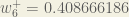
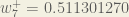
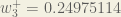
We can now update $w_1$ :

$w_1^{+} = w_1 - \eta * \frac{\partial E_{total}}{\partial w_{1}} = 0.15 - 0.5 * 0.000438568 = 0.149780716$

Repeating this for $w_2$ , $w_3$ , and $w_4$

$w_2^{+} = 0.19956143$

$w_3^{+} = 0.24975114$

$w_4^{+} = 0.29950229$

Finally, we’ve updated all of our weights! When we fed forward the 0.05 and 0.1 inputs originally, the error on the network was 0.298371109. After this first round of backpropagation, the total error is now down to 0.291027924. It might not seem like much, but after repeating this process 10,000 times, for example, the error plummets to 0.0000351085. At this point, when we feed forward 0.05 and 0.1, the two outputs neurons generate 0.015912196 (vs 0.01 target) and 0.984065734 (vs 0.99 target).

If you’ve made it this far and found any errors in any of the above or can think of any ways to make it clearer for future readers, don’t hesitate to drop me a note. Thanks!

And while I have you…

Again, if you liked this tutorial, please check out Emergent Mind, a site I’m building with an end goal of explaining AI/ML concepts in a similar style as this post. Feedback very much welcome!

1,090 thoughts on “A Step by Step Backpropagation Example”

Pingback: 1p – A Step by Step Backpropagation Example | Profit Goals
Pingback: 1p – A Step by Step Backpropagation Example – Exploding Ads
hmc says:

May 19, 2015 at 5:29 pm

Hello Matt,
It’s about three things.
When you say

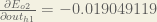
Following the same proccess for DEo2/Douto2, we get:
DEo2/Douth1 = -0.019049119

no should be
… DEo2/Douth2, we get: // h2
DEo2/Douth2 = -0.019049119 ? // h2

And in the end, when update w1+
0.000364723 this value no should
be 0.000438568 and result change
a little.

And finally
Thanks for the explanation. Very illustrative.

Reply
1. Mazur says:
  
  June 11, 2015 at 2:32 pm
  
  Hey HMC, in that part of the writeup we’re figuring out how to update w1. The output of h2 doesn’t affect w1 so I don’t think it would be included in any of the calculations; we’re only looking at h1 there. Thoughts?
  
  Reply
robfelty says:

May 22, 2015 at 6:56 pm

Nice work Matt! I love the visualizations. I have hard copies of the original neural network papers from the 80’s if you are interested some time.

Reply
Katie says:

July 3, 2015 at 1:05 am

Great post Matt! I’ve been checking out neural network tutorials on the net and really appreciate how your post actually walks through how to derive the deltas used in backpropagation (other similar tutorials all tended to just give the formula, sometimes not terribly clearly). It really sets your post apart from the others. A couple questions from a newbie trying to self-teach:

1. Is there a typo in the diagram illustrating the delta on w1? It shows partial(E_total)/partial(out_h1) = partial(E_o1)/partial(out_h1) + partial(E_o2)/partial(out_h2). Should that out_h2 in the last denominator actually be out_h1?

2. What are some typical expectations of the number of training runs needed to train up a network? Say with an eta of 0.5 as you used in your example, you casually mentioned 10k runs – is this a typical number? I ask as I’m trying to train a network on a trivially simple problem as an exercise but it just doesn’t seem to learn correctly, and it would be useful to identify if I’m just not giving it enough training runs, or if there’s something fundamentally wrong in my implementation. Apologies if this question is beyond the scope of your post, but none of the tutorials I’ve found seem to have any info on typical training run lengths, and yours was the only one that seemed interested in using actual numbers to illustrate!

Reply
1. Mazur says:
  
  July 3, 2015 at 11:57 am
  
  Hey Katie, thank you for the kudos and the pointing out the problem with that diagram. You were correct, it should have been h1 in the denominator. I updated the diagram.
  
  As for your second question, I’m not entirely sure myself. As I understand it, there’s not even a good way to determine beforehand how many hidden layer neurons you should use; it’s something you have to figure out through trial and error. It might be the same case for eta and the number of runs. You could try asking on a forum like MathOverflow to see if anyone knows. I’d love to hear the answer if you find out.
  
  Thanks again!
  
  Reply
  1. Simon Vrouwenvelder says:
    
    August 2, 2015 at 5:51 pm
    
    Hi Katie and Mat,
    
    There is indeed no way of knowing how much hidden neurons you will need ‘a priori’. However, there is a way to find one by trial and error.
    
    More neurons will always ensure that you will have a better fit for your specific dataset. However, all datasets contain noise, so your network will at some point start to fit the noise of your dataset. By introducing a validation dataset you will be able to find an optimum number of neurons that has the smallest error for the validation dataset while being trained by another dataset (the ‘original’). That is the number you should use.
    You may split your initial dataset in two parts (80/20, or 70/30) such that the 80% part is your training set and the 20% part is your validation dataset.
    
    This does not mean you have found the optimal neural network. You may change the activation functions on some nodes, or the topology for that matter. A method that does the latter is NEAT (Neuro Evolution of Augmented Topologies). ANN are at some parts more of an art than science.
    
    Reply
Pingback: matt1 comments on “A Neural Network in 11 Lines of Python” | Exploding Ads
Marco says:

July 15, 2015 at 5:33 am

Hi! First of all, thanks a lot for your post, I’m a newbie to NNs and it helped me greatly to understand the idea behind them. More than in the numbers, I’m interested in motivation, and there’s a point in your algorithm I don’t quite understand: biases.

Now, the whole concept was new to me, but googling around I understood why in general someone would like biases, see for example the answer here:
http://stackoverflow.com/questions/2480650/role-of-bias-in-neural-networks
Mathematically speaking it’s clear, in the very easy example in Stack Overflow you’d like (prior to applying the sigmoid), even with 1 input and 1 output and no hidden layers, to be allowed to use affine functions and not just linear ones, and I can see well why someone would like to do that. After all the same thing is a standard already in the much easier setting of linear regression.

For a slightly more complicated NN as yours, this makes at least as much sense in hidden layers, where the values in the middle keep changing; if you’re expecting a constant value to be added to your output (or your next layer), you definitely need some bias, the value of which stays fixed.

What I don’t get from your post, that seems to differ to the answer there, is that I don’t see you updating the weights in the biases; am I wrong about that? I would have expected the 4 arrows going out of b1 and b2 to have non-constant weights, as well, which are updated in pretty much the same way as w1, …, w8. This is because in the present form, prior to applying the sigmoid, you do have an non-linear affine function, of course, say y = ax + b. But the bias (b, the value of this affine function in x=0) is constant and immutable, equal to .35 and .6 whatever else happens in the NN; it seems to me that in this way you are just forcing your other weights to balance for these biases. In my intuition (at least for the last hidden layer) this helps if, by chance, your biases move you toward the “right” answer, but goes against you otherwise – and of course you cannot know that before training the network.

Am I wrong about something? Is adding a constant bias always useful nevertheless? Or, on the other hand, updating their weights would lead to over-fitting? If one of these two is true and you do want constant biases, how do you prescribe the values? They can’t just be any random number, if they were much bigger than the other weights and of the “right” answer, the time required for training your NN would skyrocket…

Reply
marcospinaci says:

July 15, 2015 at 5:35 am

Hi! First of all, thanks a lot for your post, I’m a newbie to NNs and it helped me greatly to understand the idea behind them. More than in the numbers, I’m interested in motivation, and there’s a point in your algorithm I don’t quite understand: biases.

Now, the whole concept was new to me, but googling around I understood why in general someone would like biases, see for example the answer here:
http://stackoverflow.com/questions/2480650/role-of-bias-in-neural-networks
Mathematically speaking it’s clear, in the very easy example in Stack Overflow you’d like (prior to applying the sigmoid), even with 1 input and 1 output and no hidden layers, to be allowed to use affine functions and not just linear ones, and I can see well why someone would like to do that. After all the same thing is a standard already in the much easier setting of linear regression.

For a slightly more complicated NN as yours, this makes at least as much sense in hidden layers, where the values in the middle keep changing and if you’re expecting a constant value to be added to your output (or your next layer), you definitely need some bias, the value of which stays fixed.

What I don’t get from your post, that seems to differ to the answer there, is that I don’t see you updating the weights in the biases; am I wrong about that? I would have expected the arrows going out of b1 and b2 to have non-constant weights, as well, which are updated in pretty much the same way as w1, …, w8. This is because in the present form, prior to applying the sigmoid, you do have an non-linear affine function, of course, say y = ax + b. But the bias (in this case b, the value of this affine function in x=0) is constant and immutable, equal to .35 and .6 whatever else happens in the NN; it seems to me that in this way you are just forcing your other weights to balance for these biases. In my intuition (at least for the last hidden layer) this helps if, by chance, your biases move you toward the “right” answer, but goes against you otherwise – and of course you cannot know that before training the network.

Am I wrong about something? Is adding a constant bias always useful nevertheless? Or, on the other hand, updating their weights would lead to over-fitting? If one of these two is true, how do you prescribe the values of biases? They can’t just be any random number, I’d say that if they were much bigger than the other weights and of the “right” answer, the time required for training your NN would skyrocket…

Reply
1. Mazur says:
  
  July 15, 2015 at 9:45 am
  
  Hey Marco, as far as I understand it you do not update the biases. I skimmed over the Stack Overflow post and didn’t notice them discussing it there, though might have missed it (if I did, please point me to where they say to do it). The backpropagation algorithm will automatically adjust the weights to minimize the error regardless of the initial values are for the biases. Hope this helps!
  
  Reply
  1. Marco says:
    
    July 15, 2015 at 10:10 am
    
    Thanks for the answer! I think the answers in SO somehow implicitly mean that it should be updated, because they call the weights of the bias with the same letters as the other ones, thus including them in the cycle of update. The second (less voted) answer is slightly more explicit, by citing (and more helpfully linking) a book where the author starts by using a non-biased NN with a translated sigmoid (1/(1+e^{-2s(x+t)}). But then, it says that the translation value t must be adjusted during the training, together with the weights; and to avoid this, it adds a new neuron, the bias, with its own weight, I guess implicitly meaning “so that you update it in the same way as the others”.
    
    The following SO question/answer is perhaps more explicit about the point, it doesn’t say “if” or “why” you should update those weights, but “how”, so again I think it is implicit that you should:
    http://stackoverflow.com/questions/3775032/how-to-update-the-bias-in-neural-network-backpropagation
    
    Let me know if you see any flaws!
    
    Reply
    1. Mazur says:
      
      July 15, 2015 at 10:43 am
      
      Now that you mention it, I seem to recall reading that in some more advanced neural network algorithms the bias is indeed updated during the training. However, for a simple neural network with backpropagation like in the post above the biases are fixed.
      
      Reply
kevincoletta says:

July 15, 2015 at 12:56 pm

Reblogged this on Kevin Coletta and commented:
Cool neural network example.

Reply
Ari Wilson says:

July 15, 2015 at 5:20 pm

I’m pretty sure you update the biases as well for effective learning. At least I ran your example with a per-neuron bias (not quite the same as your network) and after 1 iteration had training error of 0.277. After 10k iterations I was down to 1.4*10^-24.

Reply
Pingback: Bookmarks for July 14th through July 15th | Chris's Digital Detritus
russomi says:

July 16, 2015 at 5:57 am

Reblogged this on russomi.

Reply
Pingback: Distilled News | Data Analytics & R
Brian says:

July 17, 2015 at 8:02 am

Matt…Absolutely Brilliant! Thank you…

Reply
nSv says:

July 19, 2015 at 1:15 pm

Best explanation of Backpropagation so far… Thank you

Reply
Nam Khanh says:

July 20, 2015 at 8:14 am

Reblogged this on Nam Khanh Tran.

Reply
Pingback: A Step by Step Backpropagation Example | Dinesh Ram Kali.
Lauren says:

July 22, 2015 at 6:45 pm

There seems to be an error. I think a couple people pointed it out already, but I was hoping it’d be fixed because it’s leaving me rather confused.

Earlier, you have dEtotal/dw1 = .000438568. Then, when you write the update for w1, the new value of w1= w1 – n (deTotal/dw1) = .15 – .5 * .000367 … implying that deTotal/dw1 is actually equal to .000367 instead of .000438568.

Also, I think it’d be helpful if you showed the a couple of intermediate calculations for w2 as well, just the intermediate value of the deTotal/w2 would definitely be helpful.

Reply
1. Mazur says:
  
  July 23, 2015 at 3:25 pm
  
  Hey Lauren, you are absolutely correct. I understand the original commenter’s last paragraph now too :). I updated the post accordingly.
  
  If you’d like to explore the other calculations, check out the Python script linked to at the top of the post. You can throw in print() and nn.inspect() calls at various places to check your work. Let me know how else I can help.
  
  Thanks again!
  
  Reply
Luffy says:

July 25, 2015 at 4:55 am

I look the delta value for output neuron and they don’t include the negative sign
Why???

Reply
1. Mazur says:
  
  July 25, 2015 at 9:32 am
  
  Hey Luffy, check out the blue section that starts with “You’ll often see this calculation combined in the form of the delta rule” — there’s a note at the end about different conventions for including the negative sign.
  
  Reply
Saurabh Chhabra says:

July 29, 2015 at 12:41 am

Knowing hard things to a deep extent makes them easy and changes them from being hard to easy.
Awesome content.
Heads off for your knowledge and explaining capabilities.
Thanks a ton for sharing

Reply
Anonymous says:

August 2, 2015 at 8:14 am

Hi Matt,

thank you for your post! There’s one thing I can’t understand: In the gradient descent, we want to compute each partial derivatives as we consider the output changes w.r.t to each weights (variables) but in the hidden layer the changes of one weight affects the change in the next layers. Nevertheless we are just calculating how a change in a hidden weight affects the final error assuming the next weight’s layer don’t change but we are indeed changing them. It seems strange to me. Could you clarify this for me? Thx

Reply
Peter says:

August 11, 2015 at 2:44 pm

HI i’ve created a simple neuronal network in java:
https://github.com/wutzebaer/Neuronal

It has only 3 neurons; input hidden output

When the input is > 0.7 output should be 1, otherwise 0

Question1:
When i set my rate to 1 it seems to divergate fast, when i choose 0.1 it does not come to a result. Why is this, i thought a smaller rate whould just take longer.

Question2:
Why to i only get a 99% hit rate for such a simple problem? Is it not toal solveable by a neuronal network?

Question3:
the amount of neurons per layer does not seem to have much effect, but when i choose 2 or more layers the results are worse, even when learning for a long time. Why? Warent more layers better?

I’ve checked in my small project here:
https://github.com/wutzebaer/Neuronal

Reply
Pingback: How does rate layer count affect my neuronal network - BlogoSfera
Russ says:

August 14, 2015 at 6:58 am

Hi there,

This is excellent. Thank you for taking the time to explain this in such a detailed way. I wonder if it would be possible to have some clarification on a problem I have been having with backdrop? I have added an extra hidden layer with 2 neurons and a bias, so there are 12 weights (w1 to w12 plus the ones from the bias nodes) and 4 hidden nodes (h1 to h4) and I have been trying to calculate by hand the weights for w1 which is on the connection from i1 as in your diagram. The problem is I am worried I am not doing things correctly. I know there are reasons for not doing this on a problem like this, but I would just like to know how to do it in principle.

Where I get a little worried is the branch from h1 as there are connections to h3 and h4 and then cross connections from h3 and h4 to o1 and o2. I have been going crazy with the chain rule and it was going quite well but I don’t think I have got the solution correct. Would it be possible to help me with a ‘quick’ solution to just w1 under these conditions. I will persevere in the mean time. Perhaps I have missed a trick somehow.

Thanks again

Reply
1. Russ says:
  
  August 15, 2015 at 7:57 am
  
  Sorry I just calculated the answer, I am an idiot it seems! The back pass of intermediate errors was fairly obvious! Thanks again for your amazing work!
  
  Reply
joseph says:

August 28, 2015 at 5:13 pm

Hi mat great example.
Do you have an example with 2 hidden layers?
Input-Hidden-Hidden-Output?

Reply
katysei says:

August 28, 2015 at 5:16 pm

Hi mat.
do you have an example with two hidden layers?
input->hidden->hidden->output.

Reply
zxarukas says:

August 30, 2015 at 9:35 am

This post is pretty awesome and quite straightforward. It helps me a lot. Thank you.

Reply
YUTAO says:

September 2, 2015 at 10:09 am

Hi Mat, thank you for your work. I have a question here.

In your work, the error is reduced w.r.t. one data set. When we have a bunch of data that is to say, not a single training set, how can we update the weights?

I’m trying to implement the BP algorithm to a batch training problem. I have some problems how to gather the overall error of all input-output pairs and calculate the gradient.

Thank you

Reply
Anuradha Srinivas says:

September 3, 2015 at 1:10 pm

hi matt. good job. very good illustrative example.

Reply
denson smith says:

September 4, 2015 at 1:35 pm

Great tutorial!

Reply
Master says:

September 12, 2015 at 2:28 am

Great Article.
I tried implementing a simpler network (xor) to see how it really works.!
But I’ve been failing to no end!
I tried creating xor network using 3 methods:
I)with normal weights and biases
II)without any biases
II)biases as weights

None of these work in the way they should. I am not familiar with matlab, but had a look at things that would get me going and let me code, and then started coding this.

I would be grateful if you could give me a hand in this and help me find my problem.
Here is the links to my codes :
I) http://pastebin.com/jb2PAJ5u
II) http://pastebin.com/Ah09jyiw
III) http://pastebin.com/7wC5Si4V

By the way, I tried explaining what I was doing in the first version thoroughly ( the other two are the same in terms of formulation) so whoever reads the code , knows whats going on.

Thank you very much again for your time and great explanation

Reply
Marc says:

September 13, 2015 at 10:38 am

Matt, great example! This was the explanation I needed to get going!

Master I also struggled with the XOR example. I tried everything that you tried plus a few other things.

However I found Matt’s Emergent Mind #10, javascript visual. I built a NN with 5 hidden nodes as that example used and now the XOR is working fine.

Hope that helps.

Marc

Reply
Pingback: A Visual Guide to (Feed Forward) Neural Networks | mbuffett.blog()
Rajesh Bhat says:

October 4, 2015 at 5:10 am

Can anyone explain me the role bias term in neural networks?
Thanks in advance.

Reply
Viva la laMustafa (@vivalalamustafa) says:

October 5, 2015 at 4:22 am

Very nice tutorial, thanks

Reply
harsimranpal says:

October 9, 2015 at 10:36 am

Hey Mazur
I want to classify the documents into different categories by using neural networks. Please give me the step by step algorithm for classification of documents.

Reply
Syete says:

October 13, 2015 at 3:23 pm

Great post!!!!!!!!! The visualization is excellent

Thank for all !!!!

Reply
Danijar Hafner says:

October 14, 2015 at 2:30 pm

Thanks for the good article, Matt! I think we could compute the gradient with respect to all incoming activations dE/dnet first. In a second pass, we can compute gradient with respect to all weights dE/dw from that. Is that correct? I’d just like to validate my understanding.

Reply
adilla says:

October 21, 2015 at 3:09 am

thank you for your explanations..as a newbie, it really helps me to understand it better with visualization.

Reply
adilla says:

October 21, 2015 at 3:54 am

i hv a question.. are they same; 1/(1+e^(-net h1) = 1/(1+exp(-x)

Reply
Mohit says:

October 21, 2015 at 1:30 pm

Thanks matt for this post…i never understood training of neural nets before this post..thanks it helped me lot

Reply
DANIEL says:

October 25, 2015 at 12:12 am

Thanks a lot. I only have one question. When you write dnet01/douth1=w5 why do you get w5.

Reply
Sushovan says:

October 26, 2015 at 5:55 pm

Hi, I just wanted to say thank you so much for this Blog post. I am curtlnrey writing a paper on network theory and how it relates to marketing entertainment product for uni. I really loved the comparison of the two pictures they really are so alike, the more research I do the more I realize how similar all networks are and how the pertain to so many different facets of our life. My main interest is social networks and the way we connect with one another, there is a great app on facebook that can make a network map of your online friend. I found it very interesting.well thanks again.Bye

Reply
cyanogenie says:

October 26, 2015 at 10:41 pm

Thanks for the post. :)

Reply
Pingback: Introduction to Convolution Neural Networks | Infilect
Isaac Zinda says:

October 30, 2015 at 2:42 pm

This is awesome! Thanks for the great work.

Reply
Amir Bar says:

November 7, 2015 at 3:55 pm

Very very nice!!! helped me a lot to understand step by step.

Reply
Shak says:

November 19, 2015 at 5:30 pm

This is exactly the type of material I was looking for to better understand backpropagation method, thanks a lot Matt!

Reply
Shak says:

November 20, 2015 at 4:11 pm

Matt, I got a quick question: I have also seen the Error defined as SUM(target*log(output)+(1-target)*log(1-output)). Would the math come out the same way if you use this or does it complicate the things?

Reply
Nayantara says:

November 22, 2015 at 12:41 pm

Hey Matt, Amazing post! The explanation was wonderful. this is one of the best resources on the internet which explains back propagation so well – using actual values. However, I have a couple of questions :
1) The bias for both the layers – is it set to a random value ? How is the bias chosen ? Also, does the bias have to be same for both nodes of a layer ?
2) The learning rate(eta) – does it have to be same while applying gradient descent on each of the weights ?

Reply
1. Mazur says:
  
  November 23, 2015 at 8:42 am
  
  Hey Nayantara, the bias is initially random for each neuron. The learning rate is constant, but there might be some work out there that varies it to measure the impact; not sure.
  
  Reply
  1. Nayantara says:
    
    November 23, 2015 at 1:02 pm
    
    Thanks! :)
    
    Reply