Visualizing Your SaaS App’s Monthly Active Users Broken Down by Signup Cohort

This week at Automattic I’ve been helping with a tool that will allow us to visualize the number of active WordPress.com users each month broken down by when those users signed up for an account. I think this type of chart and what you can learn from it are incredibly valuable so I wanted to show you all how to quickly create one for your own service.

Here’s an example of what this type of chart looks like courtesy of Buffer’s Joel Gascoigne:

1/ Here's cohort chart of @buffer active users. Layer = signup month. Even 2 year old cohorts contribute 2k actives. pic.twitter.com/1zhsp4QgGG

— Joel Gascoigne (@joelgascoigne) October 29, 2014

What I really like about it is that for each month you can see how many active users there are and when those users signed up for an account. This not only gives you a sense how long ago your active users signed up, but also of your service’s ability to retain users over time.

If you’d like to create a similar chart to visualize your SaaS app’s active users, I put together a small R script on Github that will help you do just that.

The only thing that you need to provide the script is a CSV file that contains user IDs and dates that those users performed an action in your app.

For example, the test data set that comes with it contains user IDs and actions performed by users of one of my apps (Preceden, a web-based timeline maker) for the first year that the site existed (as determined by the automatically set created_at and updated_at values on the Ruby on Rails Active Record objects that each user is associated with):

2   2010-03-28
2   2010-04-09
2   2010-04-10
2   2010-05-16
3   2010-01-31
3   2014-05-07
3   2014-09-30
3   2015-04-11
4   2010-01-31
4   2010-10-06
...

In this example user IDs 2 and 3 each performed actions on four dates and user ID 4 performed actions on 2 dates. The script will analyze that data to figure out which cohort the user belongs to based on the earliest date the user performed an action and count that user toward the active users for each subsequent month that he or she performed an action:

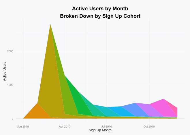
As you can see there was a huge spike at the beginning of the year when Preceden launched on HackerNews and was subsequently covered on other tech sites, but by December only a fraction of those users were still active. On that note, I encourage you to strive to build a service like Buffer that delivers long term value so your chart doesn’t wind up looking like this one :).

If you have any questions or need help customizing the script in any way, please don’t hesitate to drop me a note.

Thanks Joel Martinez and Rob Felty for providing feedback on the code.

Visualizing the Sampling Distribution of a Proportion with R

In yesterday’s post, we showed that a binomial distribution can be approximated by a normal distribution and some of the math behind it.

Today we’ll take it a step further, showing how those results can help us understand the distribution of a sample proportion.

Consider the following example:

Out of the last 250 visitors to your website, 40 signed up for an account.

The conversion rate for that group is 16%, but it’s possible (and likely!) that the true conversion rate differs from this. Statistics can help us determine a range (a confidence interval) for what the true conversion rate actually is.

Recall that in the last post we said that the mean of the binomial distribution can be approximated with a normal distribution with a mean and standard deviation calculated by:

$\mu = np$

$\sigma = \sqrt{npq}$

For a proportion, we want to figure out the mean and standard deviation on a per-trial basis so we divide each formula by n, the number of trials:

$\mu = \frac{np}{n} = p$

$\sigma = \frac{\sqrt{npq}}{n} = \sqrt{\frac{npq}{n^2}} = \sqrt{\frac{pq}{n}}$

With the mean and standard deviation of the sample proportion in hand, we can plot the distribution for this example:

As you can see, the most likely conversion rate is 16% (which is no surprise), but the true conversion rate can fall anywhere under that curve with it being less and less likely as you move farther away.

Where it gets really interesting is when you want to compare multiple proportions.

Let’s say we’re running an A/B test and the original had 40 conversions out of 250 like the example above and the experimental version had 60 conversions out of 270 participants. We can plot the distribution of both sample proportions with this code:

	setClass(
	Class = "Distribution",
	representation = representation(
	name = "character",
	participants = "numeric",
	conversions = "numeric",
	sample_proportion = "numeric",
	se = "numeric",
	color = "character",
	x = "vector",
	y = "vector"
	)
	)

	# We rewrite the initialize method for Distribution objects so that we can
	# set the x and y values which are used throughout the plotting process
	setMethod(
	f = "initialize",
	signature = "Distribution",
	definition = function( .Object, name, participants, conversions, color ) {
	.Object@name = name
	.Object@sample_proportion = conversions / participants
	.Object@se = sqrt( ( .Object@sample_proportion * ( 1 – .Object@sample_proportion ) ) / participants )
	.Object@color = color
	.Object@x = seq( –4, 4, length = 100 ) * .Object@se + .Object@sample_proportion
	.Object@y = dnorm( .Object@x, .Object@sample_proportion, .Object@se )

	return ( .Object )
	}
	)

	# Given a list of distributions, this returns a list of the x and y axis range
	get_axis_ranges = function( distributions ) {
	x_all = vector()
	y_all = vector()

	for ( distribution in distributions ) {
	x_all = c( x_all, distribution@x )
	y_all = c( y_all, distribution@y )
	}

	xlim = c( min( x_all ), max( x_all ) )
	ylim = c( min( y_all ), max( y_all ) )

	# Note that by forming a list of the vectors, the vectors get converted to lists
	# which we then have to convert back to vectors in order to use them for plotting
	return ( list( xlim, ylim ) )
	}

	get_x_axis_values = function( x_range ) {
	by = 0.01

	min_x = floor( min( x_range ) / by ) * by
	max_x = ceiling( max( x_range ) / by ) * by

	return ( seq( min_x, max_x, by = by ) )
	}

	# Define the distributions that we want to plot
	distributions = list(
	new( Class = "Distribution", name = "original", participants = 250, conversions = 40, color = "#00cc00" ),
	new( Class = "Distribution", name = "variation", participants = 270, conversions = 60, color = "blue" )
	)

	# Determine the range to use for each axis
	axis_range = get_axis_ranges( distributions )
	xlim = axis_range[[ 1 ]]
	ylim = axis_range[[ 2 ]]

	# Create the plot
	plot( NULL, NULL, type = "n", xlim = xlim, ylim = ylim, xlab = "Conversion Rate", ylab = "", main = "", axes = FALSE )

	# Render each of the curves
	line_width = 3
	for ( distribution in distributions ) {
	polygon( distribution@x, distribution@y, col = adjustcolor( distribution@color, alpha.f = 0.3 ), border = NA )
	lines( distribution@x, distribution@y, col = adjustcolor( distribution@color, alpha.f = 1 ), lwd = line_width )

	# Draw a line down the center of the curve
	ci_center_y = dnorm( distribution@sample_proportion, distribution@sample_proportion, distribution@se )
	coords = xy.coords( c( distribution@sample_proportion, distribution@sample_proportion ), c( 0, ci_center_y ) )
	lines( coords, col = adjustcolor( distribution@color, alpha.f = 0.4 ), lwd = 1 )
	}

	# Render the x axis
	axis( side = 1, at = get_x_axis_values( xlim ), pos = 0, col = "#777777", col.axis = "#777777", lwd = line_width )

	# Finally, render a legend
	legend_text = vector()
	legend_colors = vector()
	for ( distribution in distributions ) {
	legend_text = c( legend_text, distribution@name )
	legend_colors = c( legend_colors, distribution@color )
	}
	legend('right', legend_text, lty = 1, lwd = line_width, col = legend_colors, bty = 'n' )

view raw

sample-proportions.r

hosted with ❤ by GitHub

Here’s the result:

What can we determine from this? Is the experimental version better than the original? What if the true proportion for the original is 20% (towards the upper end of its distribution) and the true proportion for the experimental version is 16% (towards the lower end of its distribution)?

We’ll save the answer for a future post :)

Visualizing How a Normal Distribution Approximates a Binomial Distribution with R

My handy Elementary Statistics textbook, which I’m using to get smart on the math behind A/B testing, states the following:

Normal Distribution as Approximation to Binomial Distribution

If $np \geq 5$ and $nq \geq 5$ , then the binomial random variable has a probability distribution that can be approximated by a normal distribution with the mean and standard deviation given as:

$\mu = np$

$\sigma = \sqrt{npq}$

In easier to understand terms, take the following example:

Each visitor to your website has a 30% chance of signing up for an account. Over the next 250 visitors, how many can you expect to sign up for an account?

The first formula lets us figure out the mean by simply multiplying the number of visitors by the probability of a successful conversion:

$\mu = np = 250 * 0.30 = 75$

Simple enough and fairly easy to understand.

The second formula, the one to figure out the standard deviation, is less intuitive:

$\sigma = \sqrt{npq} = \sqrt{250 * 0.30 * (1 - 0.30)} = 7.25$

Why are we taking the square root of the product of these three values? The textbook doesn’t explain, noting that “the formal justification that allows us to use the normal distribution as an approximation to the binomial distribution results from more advanced mathematics”.

Because this standard deviation formula plays a big role in calculating the confidence intervals for sample proportions, I decided to simulate the scenario above to prove to myself that the standard deviation formula is accurate.

The R script below simulates 250 visitors coming to a website, each with a 30% chance of signing up. After each group of 250 visitors we track how many of them wound up converting. After all of the runs (the default is 1,000, though the higher the number the more accurate the distribution will be) we plot the probability distribution of the results in blue and a curve representing what we’d expect the distribution to look like if the standard deviation formula above is correct in red.

	experiments = 1000
	visitors = 250
	conversion_rate = 0.3

	expected_conversions = visitors * conversion_rate
	expected_sd = sqrt( visitors * conversion_rate * ( 1 – conversion_rate ) )
	sd_for_axis_range = 4.5
	axis_divisions = 5

	results = vector()
	for ( experiment in 1:experiments ) {
	conversions = 0
	for ( visitor in 1:visitors ) {
	if ( runif( 1 ) <= conversion_rate ) {
	conversions = conversions + 1
	}
	}
	results = c( results, conversions )
	}

	par( oma = c( 0, 2, 0, 0 ) )

	axis_min = floor( ( expected_conversions – sd_for_axis_range * expected_sd ) / axis_divisions ) * axis_divisions
	axis_max = ceiling( ( expected_conversions + sd_for_axis_range * expected_sd ) / axis_divisions ) * axis_divisions
	hist( results, axes = FALSE, breaks = seq( axis_min, axis_max, by = 1 ), ylab = 'Probability', xlab = 'Conversions', freq = FALSE, col = '#4B85ED', main = 'Distribution of Results' )

	axis( side = 1, at = seq( axis_min, axis_max, by = axis_divisions ), pos = 0, col = "#666666", col.axis = "#666666", lwd = 1, tck = –0.015 )
	axis( side = 2, col = "#666666", col.axis = "#666666", lwd = 1, tck = –0.015 )

	curve( dnorm(x, mean = conversion_rate * visitors, sd = expected_sd ), add = TRUE, col = "red", lwd = 4 )

view raw

normal-dist.r

hosted with ❤ by GitHub

The distribution of results from this experiment paints a telling picture:

Not only is the mean what we expect (around 75), but the standard deviation formula (which said it would be 7.25) does predict the standard deviation from this experiment (7.25). Go figure :)

As we’ll see, we can use the fact that the normal distribution approximates a binomial distribution approximates to figure out the distribution of a sample proportion, which we can then compare to other sample proportion distributions to make conclusions about whether they differ and by how much (ie, how to analyze the results of an A/B test).

Rendering Two Normal Distribution Curves on a Single Plot with R

As a follow-up to my last post about how to render a normal distribution curve with R, here’s how you can render two on the same plot:

setClass(
	Class = "Distribution",
	representation = representation(
		name = "character",
		mean = "numeric",
		sd = "numeric",
		color = "character",
		x = "vector",
		y = "vector"
	)
)

# We rewrite the initialize method for Distribution objects so that we can
# set the x and y values which are used throughout the plotting process
setMethod(
	f = "initialize",
	signature = "Distribution",
	definition = function( .Object, name, mean, sd, color ) {
		.Object@name = name
		.Object@mean = mean
		.Object@sd = sd
		.Object@color = color
		.Object@x = seq( -4, 4, length = 1000 ) * sd + mean
		.Object@y = dnorm( .Object@x, mean, sd )

		return ( .Object )
	}
)

# Given a list of distributions, this returns a list of the x and y axis range
get_axis_ranges = function( distributions ) {
	x_all = vector()
	y_all = vector()

	for ( distribution in distributions ) {
		x_all = c( x_all, distribution@x )
		y_all = c( y_all, distribution@y )
	}

	xlim = c( min( x_all ), max( x_all ) )
	ylim = c( min( y_all ), max( y_all ) )

	# Note that by forming a list of the vectors, the vectors get converted to lists
	# which we then have to convert back to vectors in order to use them for plotting
	return ( list( xlim, ylim ) )
}

# Define the distributions that we want to plot
distributions = list(
	new( Class = "Distribution", name = "women", mean = 63.6, sd = 2.5, color = "pink" ),
	new( Class = "Distribution", name = "men", mean = 69, sd = 2.8, color = "blue" )
)

# Determine the range to use for each axis
axis_range = get_axis_ranges( distributions )
xlim = unlist( axis_range[ 1 ] )
ylim = unlist( axis_range[ 2 ] )

# Create the plot
plot( NULL, NULL, type = "n", xlim = xlim, ylim = ylim, xlab = "Height (inches)", ylab = "", main = "Distribution of Heights", axes = FALSE )

# Render each of the curves
line_width = 3
for( distribution in distributions ) {
	lines( distribution@x, distribution@y, col = distribution@color, lwd = line_width )
}

# Render the x axis
axis_bounds <- seq( min( xlim ), max( xlim ) )
axis( side = 1, at = axis_bounds, pos = 0, col = "#aaaaaa", col.axis = "#444444" )

# Finally, render a legend
legend_text = vector()
legend_colors = vector()
for ( distribution in distributions ) {
	legend_text = c( legend_text, distribution@name )
	legend_colors = c( legend_colors, distribution@color )
}
legend('right', legend_text, lty = 1, lwd = line_width, col = legend_colors, bty = 'n' )