A Step by Step Backpropagation Example

March 17, 2015February 23, 2024Mazur

Background

Backpropagation is a common method for training a neural network. There is no shortage of papers online that attempt to explain how backpropagation works, but few that include an example with actual numbers. This post is my attempt to explain how it works with a concrete example that folks can compare their own calculations to in order to ensure they understand backpropagation correctly.

Backpropagation in Python

You can play around with a Python script that I wrote that implements the backpropagation algorithm in this Github repo.

Continue learning with Emergent Mind

If you find this tutorial useful and want to continue learning about AI/ML, I encourage you to check out Emergent Mind, a new website I’m working on that uses GPT-4 to surface and explain cutting-edge AI/ML papers:

In time, I hope to use AI to explain complex AI/ML topics on Emergent Mind in a style similar to what you’ll find in the tutorial below.

Now, on with the backpropagation tutorial…

Overview

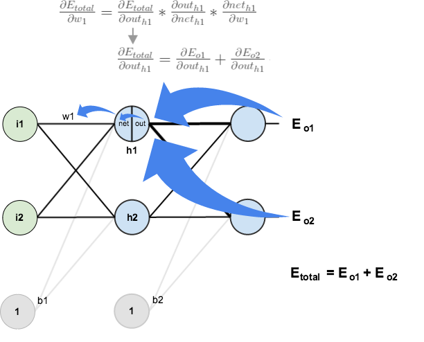
For this tutorial, we’re going to use a neural network with two inputs, two hidden neurons, two output neurons. Additionally, the hidden and output neurons will include a bias.

Here’s the basic structure:

In order to have some numbers to work with, here are the initial weights, the biases, and training inputs/outputs:

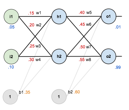
The goal of backpropagation is to optimize the weights so that the neural network can learn how to correctly map arbitrary inputs to outputs.

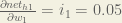
For the rest of this tutorial we’re going to work with a single training set: given inputs 0.05 and 0.10, we want the neural network to output 0.01 and 0.99.

The Forward Pass

To begin, lets see what the neural network currently predicts given the weights and biases above and inputs of 0.05 and 0.10. To do this we’ll feed those inputs forward though the network.

We figure out the total net input to each hidden layer neuron, squash the total net input using an activation function (here we use the logistic function), then repeat the process with the output layer neurons.

Total net input is also referred to as just net input by some sources.

Here’s how we calculate the total net input for $h_1$ :

$net_{h1} = w_1 * i_1 + w_2 * i_2 + b_1 * 1$

$net_{h1} = 0.15 * 0.05 + 0.2 * 0.1 + 0.35 * 1 = 0.3775$

We then squash it using the logistic function to get the output of $h_1$ :

$out_{h1} = \frac{1}{1+e^{-net_{h1}}} = \frac{1}{1+e^{-0.3775}} = 0.593269992$

Carrying out the same process for $h_2$ we get:

$out_{h2} = 0.596884378$

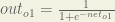
We repeat this process for the output layer neurons, using the output from the hidden layer neurons as inputs.

Here’s the output for $o_1$ :

$net_{o1} = w_5 * out_{h1} + w_6 * out_{h2} + b_2 * 1$

$net_{o1} = 0.4 * 0.593269992 + 0.45 * 0.596884378 + 0.6 * 1 = 1.105905967$

$out_{o1} = \frac{1}{1+e^{-net_{o1}}} = \frac{1}{1+e^{-1.105905967}} = 0.75136507$

And carrying out the same process for $o_2$ we get:

$out_{o2} = 0.772928465$

Calculating the Total Error

We can now calculate the error for each output neuron using the squared error function and sum them to get the total error:

$E_{total} = \sum \frac{1}{2}(target - output)^{2}$

Some sources refer to the target as the ideal and the output as the actual.

The $\frac{1}{2}$ is included so that exponent is cancelled when we differentiate later on. The result is eventually multiplied by a learning rate anyway so it doesn’t matter that we introduce a constant here [1].

For example, the target output for $o_1$ is 0.01 but the neural network output 0.75136507, therefore its error is:

$E_{o1} = \frac{1}{2}(target_{o1} - out_{o1})^{2} = \frac{1}{2}(0.01 - 0.75136507)^{2} = 0.274811083$

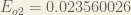
Repeating this process for $o_2$ (remembering that the target is 0.99) we get:

$E_{o2} = 0.023560026$

The total error for the neural network is the sum of these errors:

$E_{total} = E_{o1} + E_{o2} = 0.274811083 + 0.023560026 = 0.298371109$

The Backwards Pass

Our goal with backpropagation is to update each of the weights in the network so that they cause the actual output to be closer the target output, thereby minimizing the error for each output neuron and the network as a whole.

Output Layer

Consider $w_5$ . We want to know how much a change in $w_5$ affects the total error, aka $\frac{\partial E_{total}}{\partial w_{5}}$ .

$\frac{\partial E_{total}}{\partial w_{5}}$ is read as “the partial derivative of $E_{total}$ with respect to $w_{5}$ “. You can also say “the gradient with respect to $w_{5}$ ”.

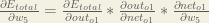
By applying the chain rule we know that:

$\frac{\partial E_{total}}{\partial w_{5}} = \frac{\partial E_{total}}{\partial out_{o1}} * \frac{\partial out_{o1}}{\partial net_{o1}} * \frac{\partial net_{o1}}{\partial w_{5}}$

Visually, here’s what we’re doing:

We need to figure out each piece in this equation.

First, how much does the total error change with respect to the output?

$E_{total} = \frac{1}{2}(target_{o1} - out_{o1})^{2} + \frac{1}{2}(target_{o2} - out_{o2})^{2}$

$\frac{\partial E_{total}}{\partial out_{o1}} = 2 * \frac{1}{2}(target_{o1} - out_{o1})^{2 - 1} * -1 + 0$

$\frac{\partial E_{total}}{\partial out_{o1}} = -(target_{o1} - out_{o1}) = -(0.01 - 0.75136507) = 0.74136507$

$-(target - out)$ is sometimes expressed as $out - target$

When we take the partial derivative of the total error with respect to $out_{o1}$ , the quantity $\frac{1}{2}(target_{o2} - out_{o2})^{2}$ becomes zero because $out_{o1}$ does not affect it which means we’re taking the derivative of a constant which is zero.

Next, how much does the output of $o_1$ change with respect to its total net input?

The partial derivative of the logistic function is the output multiplied by 1 minus the output:

$out_{o1} = \frac{1}{1+e^{-net_{o1}}}$

$\frac{\partial out_{o1}}{\partial net_{o1}} = out_{o1}(1 - out_{o1}) = 0.75136507(1 - 0.75136507) = 0.186815602$

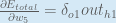
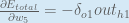
Finally, how much does the total net input of $o1$ change with respect to $w_5$ ?

$net_{o1} = w_5 * out_{h1} + w_6 * out_{h2} + b_2 * 1$

$\frac{\partial net_{o1}}{\partial w_{5}} = 1 * out_{h1} * w_5^{(1 - 1)} + 0 + 0 = out_{h1} = 0.593269992$

Putting it all together:

$\frac{\partial E_{total}}{\partial w_{5}} = \frac{\partial E_{total}}{\partial out_{o1}} * \frac{\partial out_{o1}}{\partial net_{o1}} * \frac{\partial net_{o1}}{\partial w_{5}}$

$\frac{\partial E_{total}}{\partial w_{5}} = 0.74136507 * 0.186815602 * 0.593269992 = 0.082167041$

You’ll often see this calculation combined in the form of the delta rule:

$\frac{\partial E_{total}}{\partial w_{5}} = -(target_{o1} - out_{o1}) * out_{o1}(1 - out_{o1}) * out_{h1}$

Alternatively, we have $\frac{\partial E_{total}}{\partial out_{o1}}$ and $\frac{\partial out_{o1}}{\partial net_{o1}}$ which can be written as $\frac{\partial E_{total}}{\partial net_{o1}}$ , aka $\delta_{o1}$ (the Greek letter delta) aka the node delta. We can use this to rewrite the calculation above:

$\delta_{o1} = \frac{\partial E_{total}}{\partial out_{o1}} * \frac{\partial out_{o1}}{\partial net_{o1}} = \frac{\partial E_{total}}{\partial net_{o1}}$

$\delta_{o1} = -(target_{o1} - out_{o1}) * out_{o1}(1 - out_{o1})$

Therefore:

$\frac{\partial E_{total}}{\partial w_{5}} = \delta_{o1} out_{h1}$

Some sources extract the negative sign from $\delta$ so it would be written as:

$\frac{\partial E_{total}}{\partial w_{5}} = -\delta_{o1} out_{h1}$

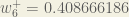
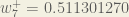
To decrease the error, we then subtract this value from the current weight (optionally multiplied by some learning rate, eta, which we’ll set to 0.5):

$w_5^{+} = w_5 - \eta * \frac{\partial E_{total}}{\partial w_{5}} = 0.4 - 0.5 * 0.082167041 = 0.35891648$

Some sources use $\alpha$ (alpha) to represent the learning rate, others use $\eta$ (eta), and others even use $\epsilon$ (epsilon).

We can repeat this process to get the new weights $w_6$ , $w_7$ , and $w_8$ :

$w_6^{+} = 0.408666186$

$w_7^{+} = 0.511301270$

$w_8^{+} = 0.561370121$

We perform the actual updates in the neural network after we have the new weights leading into the hidden layer neurons (ie, we use the original weights, not the updated weights, when we continue the backpropagation algorithm below).

Hidden Layer

Next, we’ll continue the backwards pass by calculating new values for $w_1$ , $w_2$ , $w_3$ , and $w_4$ .

Big picture, here’s what we need to figure out:

$\frac{\partial E_{total}}{\partial w_{1}} = \frac{\partial E_{total}}{\partial out_{h1}} * \frac{\partial out_{h1}}{\partial net_{h1}} * \frac{\partial net_{h1}}{\partial w_{1}}$

Visually:

We’re going to use a similar process as we did for the output layer, but slightly different to account for the fact that the output of each hidden layer neuron contributes to the output (and therefore error) of multiple output neurons. We know that $out_{h1}$ affects both $out_{o1}$ and $out_{o2}$ therefore the $\frac{\partial E_{total}}{\partial out_{h1}}$ needs to take into consideration its effect on the both output neurons:

$\frac{\partial E_{total}}{\partial out_{h1}} = \frac{\partial E_{o1}}{\partial out_{h1}} + \frac{\partial E_{o2}}{\partial out_{h1}}$

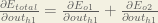
Starting with $\frac{\partial E_{o1}}{\partial out_{h1}}$ :

$\frac{\partial E_{o1}}{\partial out_{h1}} = \frac{\partial E_{o1}}{\partial net_{o1}} * \frac{\partial net_{o1}}{\partial out_{h1}}$

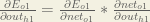
We can calculate $\frac{\partial E_{o1}}{\partial net_{o1}}$ using values we calculated earlier:

$\frac{\partial E_{o1}}{\partial net_{o1}} = \frac{\partial E_{o1}}{\partial out_{o1}} * \frac{\partial out_{o1}}{\partial net_{o1}} = 0.74136507 * 0.186815602 = 0.138498562$

And $\frac{\partial net_{o1}}{\partial out_{h1}}$ is equal to $w_5$ :

$net_{o1} = w_5 * out_{h1} + w_6 * out_{h2} + b_2 * 1$

$\frac{\partial net_{o1}}{\partial out_{h1}} = w_5 = 0.40$

Plugging them in:

$\frac{\partial E_{o1}}{\partial out_{h1}} = \frac{\partial E_{o1}}{\partial net_{o1}} * \frac{\partial net_{o1}}{\partial out_{h1}} = 0.138498562 * 0.40 = 0.055399425$

Following the same process for $\frac{\partial E_{o2}}{\partial out_{h1}}$ , we get:

$\frac{\partial E_{o2}}{\partial out_{h1}} = -0.019049119$

Therefore:

$\frac{\partial E_{total}}{\partial out_{h1}} = \frac{\partial E_{o1}}{\partial out_{h1}} + \frac{\partial E_{o2}}{\partial out_{h1}} = 0.055399425 + -0.019049119 = 0.036350306$

Now that we have $\frac{\partial E_{total}}{\partial out_{h1}}$ , we need to figure out $\frac{\partial out_{h1}}{\partial net_{h1}}$ and then $\frac{\partial net_{h1}}{\partial w}$ for each weight:

$out_{h1} = \frac{1}{1+e^{-net_{h1}}}$

$\frac{\partial out_{h1}}{\partial net_{h1}} = out_{h1}(1 - out_{h1}) = 0.59326999(1 - 0.59326999 ) = 0.241300709$

We calculate the partial derivative of the total net input to $h_1$ with respect to $w_1$ the same as we did for the output neuron:

$net_{h1} = w_1 * i_1 + w_3 * i_2 + b_1 * 1$

$\frac{\partial net_{h1}}{\partial w_1} = i_1 = 0.05$

Putting it all together:

$\frac{\partial E_{total}}{\partial w_{1}} = \frac{\partial E_{total}}{\partial out_{h1}} * \frac{\partial out_{h1}}{\partial net_{h1}} * \frac{\partial net_{h1}}{\partial w_{1}}$

$\frac{\partial E_{total}}{\partial w_{1}} = 0.036350306 * 0.241300709 * 0.05 = 0.000438568$

You might also see this written as:

$\frac{\partial E_{total}}{\partial w_{1}} = (\sum\limits_{o}{\frac{\partial E_{total}}{\partial out_{o}} * \frac{\partial out_{o}}{\partial net_{o}} * \frac{\partial net_{o}}{\partial out_{h1}}}) * \frac{\partial out_{h1}}{\partial net_{h1}} * \frac{\partial net_{h1}}{\partial w_{1}}$

$\frac{\partial E_{total}}{\partial w_{1}} = (\sum\limits_{o}{\delta_{o} * w_{ho}}) * out_{h1}(1 - out_{h1}) * i_{1}$

$\frac{\partial E_{total}}{\partial w_{1}} = \delta_{h1}i_{1}$

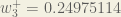
We can now update $w_1$ :

$w_1^{+} = w_1 - \eta * \frac{\partial E_{total}}{\partial w_{1}} = 0.15 - 0.5 * 0.000438568 = 0.149780716$

Repeating this for $w_2$ , $w_3$ , and $w_4$

$w_2^{+} = 0.19956143$

$w_3^{+} = 0.24975114$

$w_4^{+} = 0.29950229$

Finally, we’ve updated all of our weights! When we fed forward the 0.05 and 0.1 inputs originally, the error on the network was 0.298371109. After this first round of backpropagation, the total error is now down to 0.291027924. It might not seem like much, but after repeating this process 10,000 times, for example, the error plummets to 0.0000351085. At this point, when we feed forward 0.05 and 0.1, the two outputs neurons generate 0.015912196 (vs 0.01 target) and 0.984065734 (vs 0.99 target).

If you’ve made it this far and found any errors in any of the above or can think of any ways to make it clearer for future readers, don’t hesitate to drop me a note. Thanks!

And while I have you…

Again, if you liked this tutorial, please check out Emergent Mind, a site I’m building with an end goal of explaining AI/ML concepts in a similar style as this post. Feedback very much welcome!

1,111 thoughts on “A Step by Step Backpropagation Example”

Abhi says:

February 29, 2016 at 5:48 am

Very nicely and precisely explained. It is all to the point. Thank you :)

Reply
falcatrua says:

February 29, 2016 at 2:23 pm

It’s a great tutorial but I think I found an error:
at forward pass values should be:
neth1 = 0.15 * 0.05 + 0.25 * 0.1 + 0.35 * 1 = 0.3825
outh1 = 1/(1 + e^-0.3825) = 0,594475931
neth2 = 0.20 * 0.05 + 0.30 * 0.1 + 0.35 * 1 = 0.39
outh2 = 1/(1 + e^-0.39) = 0.596282699

Reply
1. Garett Ridge AndThenSomeMoreWords says:
  
  March 1, 2016 at 9:37 pm
  
  The labels go the other way in his drawing, where the label that says w_2 goes with the line it’s next to (on the right of it) and the value of w_2 gets written to the left; look at the previous drawing without the values to see what I mean
  
  Reply
Bill says:

March 2, 2016 at 3:09 am

Good stuff ! Professors should learn from you. Most professors make complex things complex. A real good teacher should make complex things simple.

Reply
b says:

March 2, 2016 at 3:11 am

Also , recommend this link if you want to find a even simpler example than this one. http://www.cs.toronto.edu/~tijmen/csc321/inclass/140123.pdf

Reply
Priti says:

March 2, 2016 at 4:27 am

Can you give an example for backpropagation in optical networks

Reply
Moboluwarin says:

March 2, 2016 at 2:13 pm

Hey there very helpful indeed, in the line for net01 = w5*outh1 + ‘w6’*outh2+b2*1, is it not meant to be ‘w7’ ??
Cheers

Reply
Dara says:

March 4, 2016 at 9:17 am

Can anyway help me explaining manual calculation for testing outputs with trained weights and bias? Seems it does not give the correct answer when I directly substitute my inputs to the equations. Answers are different than I get from MATLAB NN toolbox.

Reply
alaan says:

March 11, 2016 at 5:41 pm

Hello, A Step by Step Backpropagation Example is helpful. I would like to ask……What are the advantages of using the weights and biases in neural network and how the weight and biases are initialized? based on what and how?
Thanks.

Reply
sumit says:

March 13, 2016 at 3:30 am

Awesome tutorial. It clears my all doubts about Backpropagation learning algorithm. Thanks for such a nice tutorial…

Reply
Birger Skogeng Pedersen says:

March 19, 2016 at 11:05 am

This guide was incredibly helpful! I’m truly in your debt for this one, Matt.

Reply
JB says:

March 21, 2016 at 11:59 am

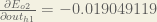
How was d(Eo2)/d(out h1)=-.019049119 calculated? thank you

Reply
JB says:

March 21, 2016 at 12:40 pm

got it…ok -.217..*.1755…*.5 =-.019….jb

Reply
Tharindu Bandara says:

March 22, 2016 at 2:02 pm

Wow you saved the day man. Literally :)

Reply
Pingback: Redes Neuronales Artificiales – Retropropagación – Nandezgarcia
Gabriel says:

March 23, 2016 at 8:31 pm

Thanks a bunch… by far the most down to earth explanation for backprop i found in a while.

Reply
Pingback: 七步理解深度学习 – Bin Zhu
Oguz says:

March 25, 2016 at 6:18 am

At the beginning, while calculating neth1, the term 0.2*0.1 should be 0.25*0.1. I do not know this changes all the numbers.

Even if all the numbers are wrong, the explanation is excellent. Thanks.

Reply
Tarun says:

March 25, 2016 at 2:37 pm

awesome article !! I have just one doubt…while calculating delta o1 , shouldn’t we multiply the given equation by weight matrix of layer 2 ? I saw that in Andrew N.Gs videos he does this and am hence confused

Reply
1. alex hao says:
  
  June 3, 2016 at 6:17 am
  
  Think you ,papi! This is the best explanation about bp I have ever seen.
  
  Reply
Pingback: Machine Learning : Resources | New Technology Information
Diego Domenech says:

March 27, 2016 at 8:44 pm

Thanks a lot, best explanation I’ve seen about backpropagation

Reply
Lavanya says:

March 28, 2016 at 11:47 am

Hey Matt, that was a very neat explanation! I am workin on BPA for SIMO system and tryin to implement using Simulink.

Is there any easy way to do in simulink?

Reply
111 says:

March 29, 2016 at 3:15 am

Thanks a ton!!!!!!

Reply
Trương Ngọc Quyền says:

March 29, 2016 at 11:28 pm

thanks a lot for this lesson!!

Reply
1. Tariq says:
  
  March 30, 2016 at 5:00 pm
  
  my guide is now published – it aims to make understanding how neural networks work as accessible as possible – with lots of diagrams, examples and discussion – there are even fun experiments to “see inside the mind of a neural network” and getting it all working on a Raspberry Pi Zero (£4 or $5)
  
  Reply
  1. Tariq says:
    
    March 30, 2016 at 5:01 pm
    
    forgot the link!
    
    Reply
    1. Flipperty says:
      
      March 30, 2016 at 6:44 pm
      
      I’ll be buying your book–it’s a great idea and well executed; but, I was hoping you could walk me through the differentiation of the total error function on pages 94-95 in the draft pdf version online. A minus that pops up that I can’t account for. The same happens in the above post, and I’m just not sure why.
      Any hep you can provide is much appreciated.
      
      Reply
      1. Tariq says:
        
        March 30, 2016 at 8:58 pm
        
        The minus sign pops up because d/dx (a-x) is -1.
        
        In the example we have d/dx (a-x)^2 which is done in two steps. First the power rule to get 2*(a-x) but then the inside of the brackets too which gives you the extra linux sign.
        
        This is actually the chain rule: df/dx = df/dy * dy/dx
        so if f=(a-x)^2 and y=(a-x) then df/dx = df/dy * dy/dx = 2y * (-1) = (a-x) * (-1)
        
        =================
        
        Some people also get caught out by the weight updates. The weights are changed in proportion to – dE/dw .. that minus is there so that the weights go in the opposite direction of the gradient. My book illustrates this too with pictures.
        
        Reply
        
        Flipperty says:
        
        March 30, 2016 at 9:04 pm
        
        Thank you! That’s what I thought, but I just needed confirmation. A lot of people don’t mention the chain rule, so that’s what was throwing me.
        
        Your book is excellent, and I bought a copy.
        
        Everybody should buy a copy!
        
        I hope it does really well.
        
        Tariq says:
        
        March 30, 2016 at 9:07 pm
        
        Thanks Flipperty – if you like it, please do leave a review on amazon. And if you have suggestions for improvement, do let me know too!
Amitesh says:

April 3, 2016 at 11:11 am

Hi Matt! Great article,probably the best I’ve come across on the internet for Backpropagation. Just noticed a small error – When you calculate outo1 for the first time in the forward pass, the formula should be 1/1-(e^-neto1) whereas you have written it to be 1/1-(e^neth1). That’s it! Amazing article once again. You’ve got me hooked on to NNets now and earned yourself a worshipper :)

Reply
1. Mazur says:
  
  April 23, 2016 at 7:44 pm
  
  Thank you (and the others) for pointing this out. Fixed!
  
  Reply
Daniel Shih says:

April 3, 2016 at 12:44 pm

Typo: At the step: out_o1 = 1/(1+exp(-net_h1)), the net_h1 should be net_o1. Right?

Reply
Mohammad ElNesr says:

April 10, 2016 at 12:00 pm

Thank you Matt for this deep explanation
I would like to ask about the bias
1- Why you set it fixed per layer, not per neuron?
2- why it is kept fixed throughout the operation, i.e., why it is not updated through the back propagation?

Thanks in advance for reply?

Reply
imaginescience says:

April 10, 2016 at 6:51 pm

Thanks a lot Matt!!

The tutorial was really great and It was really nice how you explained the concept so clearly without leaving the math out.

I had question:

When the NN trains for Example 1 and good weights are found for it. Afterwards, when the NN starts to learn for the Example 2. Will it move away from the Example 1 or will it keep accommodating it also along with Example 2 etc?

Reply
Swapnil Kumar says:

April 11, 2016 at 9:39 pm

Thank you for very clear explanation.

Reply
Rizky Yoga Oktora says:

April 13, 2016 at 4:51 am

good explanation, and easy for me to understand. thank you for your effort to explain. I appreciate this

Reply
Tarık says:

April 14, 2016 at 4:57 am

Thanks a lot for clear explanation…

Reply
joseph says:

April 18, 2016 at 2:39 am

Hi mat, Thanks for the clear explanation, one question , why don’t you use weights for the biases and update then during backprop?
thanks
joseph

Reply
katysei says:

April 18, 2016 at 2:40 am

Hi Mat, why aren’t you putting weights on biases and update them during back prop?
thanks
joseph

Reply
YB Kim says:

April 20, 2016 at 9:04 pm

Thanks for your nice post!

I have a question.

In the forward pass, there are
”
Here’s the output for o_1:

net_{o1} = w_5 * out_{h1} + w_6 * out_{h2} + b_2 * 1

net_{o1} = 0.4 * 0.593269992 + 0.45 * 0.596884378 + 0.6 * 1 = 1.105905967

out_{o1} = \frac{1}{1+e^{-net_{h1}}} = \frac{1}{1+e^{-1.105905967}} = 0.75136507
”

In my opinion, “out_{o1} = \frac{1}{1+e^{-net_{h1}}}” should be changed to
“out_{o1} = \frac{1}{1+e^{-net_{o1}}}” .

Is it right suggestion?

Reply
Jack Geng says:

April 21, 2016 at 10:13 pm

Excellent Job!

Reply
Mengü Nazlı says:

April 27, 2016 at 2:03 pm

I still see the typo here, is there a revised version of this page or you just missed it?

Reply
1. Mazur says:
  
  April 29, 2016 at 9:45 pm
  
  Thanks, that was very helpful. Fixed!
  
  Reply
kanika says:

May 1, 2016 at 10:33 am

This was an amazing tutorial! Thank you :)

Reply
Kanika Rawat says:

May 1, 2016 at 10:34 am

This was an amazing tutorial. Thank you :)

Reply
Pingback: 7 Steps to Understanding Deep Learning | Love, learn and laugh
Flemming Thomsen says:

May 4, 2016 at 6:28 am

I’m new to AI and for that reason I have traveled the net for an understandable explanation/tutorial on Back propagation. Found a lot moor or less understandable (I’m not a mathematician). I fail every time when we have to back propagate the signals. My calculus understanding was to weak. Your introduction with the chain rule together with the example with real numbers was a break through in my understanding. Thank you!

Reply
Dara says:

May 6, 2016 at 12:48 pm

Hi Mazur, this is great. I have question about this.
Doesn’t it map the training output before calculate the error with target value?. Because “logistic function” outputs are always between 0 and 1. Then what happen if my target is really high (eg:300)? error would be really high?. After finish training, my target is 300 and final output would be somewhere between 0 and 1, since transfer function at the output node is “logistic”. That is the part which I still cannot understand. even after training, doesn’t it map the output to be large (should be taken near to 300 from 0-1)?

Reply
1. @myoneuralnet says:
  
  May 6, 2016 at 1:40 pm
  
  You should map your desired outputs to match the activation function – otherwise you will drive the network to saturation. The same is also true of the inputs – you should try to optimise them to that they match the region of greatest variation of the activation function .. some people call this normalisation. My gentle intro to neural networks has a section on this .. http://www.amazon.com/dp/B01EER4Z4G
  
  Reply
John says:

May 7, 2016 at 11:05 am

Hey Mazur, great tutorial, as said earlier, the best on Internet. Just have a question, when you have more hidden layers, the concept for the feedforward is the same, but the derivatives surely will modify, my question is how to calculate it? It will be something like Dtotal = DTotal/Dout * Dout/Dnet * Dnet/Dweight * Dweight/Douthidden * Douthidden/Dnethidden * Dnethidden/Dweight? Don’t know if you will understand the way i wrote it xD Thanks in advance.

Reply
roberto brunialti says:

May 9, 2016 at 2:38 am

Thanks Matt for the great article. Even me, a math dummy, was able to implement the back prop algorithm in C++…
I’m worring abaout generalization of this algorithm: is it viable for networks with more than an hidden layer? It seems to me that the hidden part of the algorithm
is specific for jus one layer.

Reply
1. Krisztián says:
  
  May 15, 2016 at 5:25 am
  
  Theoretically only one hidden layer is enough for approximating any function, there is no need for more than an hidden layer.
  
  Reply
  1. sar33 says:
    
    July 20, 2016 at 1:22 pm
    
    True, but the key word here is “theory.” In practice, using one enormous layer is vastly inefficient and prone to runaway numerical errors. In practice, always use multiple (smaller) layers if your models need a large representational capacity.
    
    Reply
mehmet says:

May 11, 2016 at 5:46 pm

This is wonderful. Thks a lot.

Reply
hshallcross says:

May 13, 2016 at 2:08 pm

Great article Matt, thanks! How do the bias parameters of each neurone come into play with regards to back propagation?

Reply
Fengchun Qiao (@FengchunQiao) says:

May 16, 2016 at 8:13 am

clear explantion,thank u!

Reply
qwerty says:

May 17, 2016 at 12:40 am

I have a question on calculating ∂Eo1/∂ω1 using the chain rule. Eo1 is associated with both of outh1 and outh2. In your calculation, however, only the ∂neto1/∂outh1 is taken into account without consideration for ∂neto1/∂outh2. Could you explain why ∂neto1/∂outh2 can be ignored in computation?

Reply
1. sigmoid says:
  
  May 19, 2016 at 11:25 am
  
  hi qwerty, im not 100% sure with this but im guessing that w1 is not directly related to H2 that’s why. And since youre only computing for the rate of change of Eo1 with respect to change in w1, dNeto1/dOuth2 would just like be a constant/negligible.
  
  Reply
George Undefined Vlahakis says:

May 20, 2016 at 5:52 pm

Thank you. Finally something putting the theory into figures for all to understand! Next to understand layering ;-)

Reply
silvio says:

May 20, 2016 at 7:13 pm

Thank you. It help me a lot.

Reply
CrazyDiamond says:

May 21, 2016 at 3:51 pm

Thank you so much for awesome tutorial. Is there such a tutorial for the matrix form ?

Reply
ZZD says:

May 22, 2016 at 4:29 am

does b1,b2 need to be updated ?

Reply