A Step by Step Backpropagation Example

March 17, 2015February 23, 2024Mazur

Background

Backpropagation is a common method for training a neural network. There is no shortage of papers online that attempt to explain how backpropagation works, but few that include an example with actual numbers. This post is my attempt to explain how it works with a concrete example that folks can compare their own calculations to in order to ensure they understand backpropagation correctly.

Backpropagation in Python

You can play around with a Python script that I wrote that implements the backpropagation algorithm in this Github repo.

Continue learning with Emergent Mind

If you find this tutorial useful and want to continue learning about AI/ML, I encourage you to check out Emergent Mind, a new website I’m working on that uses GPT-4 to surface and explain cutting-edge AI/ML papers:

In time, I hope to use AI to explain complex AI/ML topics on Emergent Mind in a style similar to what you’ll find in the tutorial below.

Now, on with the backpropagation tutorial…

Overview

For this tutorial, we’re going to use a neural network with two inputs, two hidden neurons, two output neurons. Additionally, the hidden and output neurons will include a bias.

Here’s the basic structure:

In order to have some numbers to work with, here are the initial weights, the biases, and training inputs/outputs:

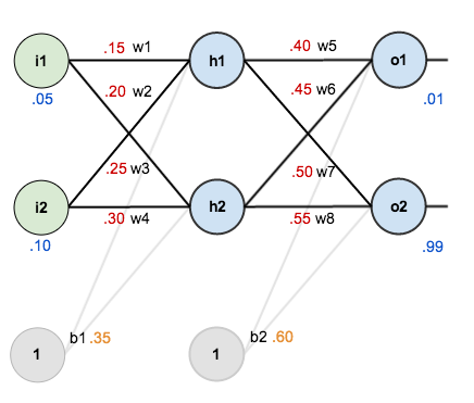
The goal of backpropagation is to optimize the weights so that the neural network can learn how to correctly map arbitrary inputs to outputs.

For the rest of this tutorial we’re going to work with a single training set: given inputs 0.05 and 0.10, we want the neural network to output 0.01 and 0.99.

The Forward Pass

To begin, lets see what the neural network currently predicts given the weights and biases above and inputs of 0.05 and 0.10. To do this we’ll feed those inputs forward though the network.

We figure out the total net input to each hidden layer neuron, squash the total net input using an activation function (here we use the logistic function), then repeat the process with the output layer neurons.

Total net input is also referred to as just net input by some sources.

Here’s how we calculate the total net input for $h_1$ :

$net_{h1} = w_1 * i_1 + w_2 * i_2 + b_1 * 1$

$net_{h1} = 0.15 * 0.05 + 0.2 * 0.1 + 0.35 * 1 = 0.3775$

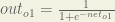
We then squash it using the logistic function to get the output of $h_1$ :

$out_{h1} = \frac{1}{1+e^{-net_{h1}}} = \frac{1}{1+e^{-0.3775}} = 0.593269992$

Carrying out the same process for $h_2$ we get:

$out_{h2} = 0.596884378$

We repeat this process for the output layer neurons, using the output from the hidden layer neurons as inputs.

Here’s the output for $o_1$ :

$net_{o1} = w_5 * out_{h1} + w_6 * out_{h2} + b_2 * 1$

$net_{o1} = 0.4 * 0.593269992 + 0.45 * 0.596884378 + 0.6 * 1 = 1.105905967$

$out_{o1} = \frac{1}{1+e^{-net_{o1}}} = \frac{1}{1+e^{-1.105905967}} = 0.75136507$

And carrying out the same process for $o_2$ we get:

$out_{o2} = 0.772928465$

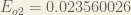
Calculating the Total Error

We can now calculate the error for each output neuron using the squared error function and sum them to get the total error:

$E_{total} = \sum \frac{1}{2}(target - output)^{2}$

Some sources refer to the target as the ideal and the output as the actual.

The $\frac{1}{2}$ is included so that exponent is cancelled when we differentiate later on. The result is eventually multiplied by a learning rate anyway so it doesn’t matter that we introduce a constant here [1].

For example, the target output for $o_1$ is 0.01 but the neural network output 0.75136507, therefore its error is:

$E_{o1} = \frac{1}{2}(target_{o1} - out_{o1})^{2} = \frac{1}{2}(0.01 - 0.75136507)^{2} = 0.274811083$

Repeating this process for $o_2$ (remembering that the target is 0.99) we get:

$E_{o2} = 0.023560026$

The total error for the neural network is the sum of these errors:

$E_{total} = E_{o1} + E_{o2} = 0.274811083 + 0.023560026 = 0.298371109$

The Backwards Pass

Our goal with backpropagation is to update each of the weights in the network so that they cause the actual output to be closer the target output, thereby minimizing the error for each output neuron and the network as a whole.

Output Layer

Consider $w_5$ . We want to know how much a change in $w_5$ affects the total error, aka $\frac{\partial E_{total}}{\partial w_{5}}$ .

$\frac{\partial E_{total}}{\partial w_{5}}$ is read as “the partial derivative of $E_{total}$ with respect to $w_{5}$ “. You can also say “the gradient with respect to $w_{5}$ ”.

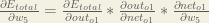
By applying the chain rule we know that:

$\frac{\partial E_{total}}{\partial w_{5}} = \frac{\partial E_{total}}{\partial out_{o1}} * \frac{\partial out_{o1}}{\partial net_{o1}} * \frac{\partial net_{o1}}{\partial w_{5}}$

Visually, here’s what we’re doing:

We need to figure out each piece in this equation.

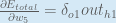
First, how much does the total error change with respect to the output?

$E_{total} = \frac{1}{2}(target_{o1} - out_{o1})^{2} + \frac{1}{2}(target_{o2} - out_{o2})^{2}$

$\frac{\partial E_{total}}{\partial out_{o1}} = 2 * \frac{1}{2}(target_{o1} - out_{o1})^{2 - 1} * -1 + 0$

$\frac{\partial E_{total}}{\partial out_{o1}} = -(target_{o1} - out_{o1}) = -(0.01 - 0.75136507) = 0.74136507$

$-(target - out)$ is sometimes expressed as $out - target$

When we take the partial derivative of the total error with respect to $out_{o1}$ , the quantity $\frac{1}{2}(target_{o2} - out_{o2})^{2}$ becomes zero because $out_{o1}$ does not affect it which means we’re taking the derivative of a constant which is zero.

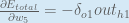
Next, how much does the output of $o_1$ change with respect to its total net input?

The partial derivative of the logistic function is the output multiplied by 1 minus the output:

$out_{o1} = \frac{1}{1+e^{-net_{o1}}}$

$\frac{\partial out_{o1}}{\partial net_{o1}} = out_{o1}(1 - out_{o1}) = 0.75136507(1 - 0.75136507) = 0.186815602$

Finally, how much does the total net input of $o1$ change with respect to $w_5$ ?

$net_{o1} = w_5 * out_{h1} + w_6 * out_{h2} + b_2 * 1$

$\frac{\partial net_{o1}}{\partial w_{5}} = 1 * out_{h1} * w_5^{(1 - 1)} + 0 + 0 = out_{h1} = 0.593269992$

Putting it all together:

$\frac{\partial E_{total}}{\partial w_{5}} = \frac{\partial E_{total}}{\partial out_{o1}} * \frac{\partial out_{o1}}{\partial net_{o1}} * \frac{\partial net_{o1}}{\partial w_{5}}$

$\frac{\partial E_{total}}{\partial w_{5}} = 0.74136507 * 0.186815602 * 0.593269992 = 0.082167041$

You’ll often see this calculation combined in the form of the delta rule:

$\frac{\partial E_{total}}{\partial w_{5}} = -(target_{o1} - out_{o1}) * out_{o1}(1 - out_{o1}) * out_{h1}$

Alternatively, we have $\frac{\partial E_{total}}{\partial out_{o1}}$ and $\frac{\partial out_{o1}}{\partial net_{o1}}$ which can be written as $\frac{\partial E_{total}}{\partial net_{o1}}$ , aka $\delta_{o1}$ (the Greek letter delta) aka the node delta. We can use this to rewrite the calculation above:

$\delta_{o1} = \frac{\partial E_{total}}{\partial out_{o1}} * \frac{\partial out_{o1}}{\partial net_{o1}} = \frac{\partial E_{total}}{\partial net_{o1}}$

$\delta_{o1} = -(target_{o1} - out_{o1}) * out_{o1}(1 - out_{o1})$

Therefore:

$\frac{\partial E_{total}}{\partial w_{5}} = \delta_{o1} out_{h1}$

Some sources extract the negative sign from $\delta$ so it would be written as:

$\frac{\partial E_{total}}{\partial w_{5}} = -\delta_{o1} out_{h1}$

To decrease the error, we then subtract this value from the current weight (optionally multiplied by some learning rate, eta, which we’ll set to 0.5):

$w_5^{+} = w_5 - \eta * \frac{\partial E_{total}}{\partial w_{5}} = 0.4 - 0.5 * 0.082167041 = 0.35891648$

Some sources use $\alpha$ (alpha) to represent the learning rate, others use $\eta$ (eta), and others even use $\epsilon$ (epsilon).

We can repeat this process to get the new weights $w_6$ , $w_7$ , and $w_8$ :

$w_6^{+} = 0.408666186$

$w_7^{+} = 0.511301270$

$w_8^{+} = 0.561370121$

We perform the actual updates in the neural network after we have the new weights leading into the hidden layer neurons (ie, we use the original weights, not the updated weights, when we continue the backpropagation algorithm below).

Hidden Layer

Next, we’ll continue the backwards pass by calculating new values for $w_1$ , $w_2$ , $w_3$ , and $w_4$ .

Big picture, here’s what we need to figure out:

$\frac{\partial E_{total}}{\partial w_{1}} = \frac{\partial E_{total}}{\partial out_{h1}} * \frac{\partial out_{h1}}{\partial net_{h1}} * \frac{\partial net_{h1}}{\partial w_{1}}$

Visually:

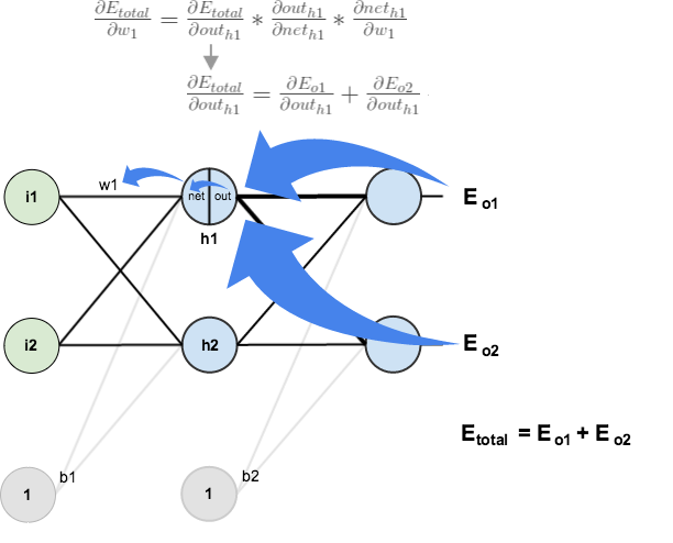
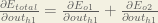
We’re going to use a similar process as we did for the output layer, but slightly different to account for the fact that the output of each hidden layer neuron contributes to the output (and therefore error) of multiple output neurons. We know that $out_{h1}$ affects both $out_{o1}$ and $out_{o2}$ therefore the $\frac{\partial E_{total}}{\partial out_{h1}}$ needs to take into consideration its effect on the both output neurons:

$\frac{\partial E_{total}}{\partial out_{h1}} = \frac{\partial E_{o1}}{\partial out_{h1}} + \frac{\partial E_{o2}}{\partial out_{h1}}$

Starting with $\frac{\partial E_{o1}}{\partial out_{h1}}$ :

$\frac{\partial E_{o1}}{\partial out_{h1}} = \frac{\partial E_{o1}}{\partial net_{o1}} * \frac{\partial net_{o1}}{\partial out_{h1}}$

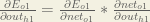
We can calculate $\frac{\partial E_{o1}}{\partial net_{o1}}$ using values we calculated earlier:

$\frac{\partial E_{o1}}{\partial net_{o1}} = \frac{\partial E_{o1}}{\partial out_{o1}} * \frac{\partial out_{o1}}{\partial net_{o1}} = 0.74136507 * 0.186815602 = 0.138498562$

And $\frac{\partial net_{o1}}{\partial out_{h1}}$ is equal to $w_5$ :

$net_{o1} = w_5 * out_{h1} + w_6 * out_{h2} + b_2 * 1$

$\frac{\partial net_{o1}}{\partial out_{h1}} = w_5 = 0.40$

Plugging them in:

$\frac{\partial E_{o1}}{\partial out_{h1}} = \frac{\partial E_{o1}}{\partial net_{o1}} * \frac{\partial net_{o1}}{\partial out_{h1}} = 0.138498562 * 0.40 = 0.055399425$

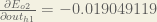
Following the same process for $\frac{\partial E_{o2}}{\partial out_{h1}}$ , we get:

$\frac{\partial E_{o2}}{\partial out_{h1}} = -0.019049119$

Therefore:

$\frac{\partial E_{total}}{\partial out_{h1}} = \frac{\partial E_{o1}}{\partial out_{h1}} + \frac{\partial E_{o2}}{\partial out_{h1}} = 0.055399425 + -0.019049119 = 0.036350306$

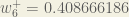
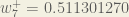
Now that we have $\frac{\partial E_{total}}{\partial out_{h1}}$ , we need to figure out $\frac{\partial out_{h1}}{\partial net_{h1}}$ and then $\frac{\partial net_{h1}}{\partial w}$ for each weight:

$out_{h1} = \frac{1}{1+e^{-net_{h1}}}$

$\frac{\partial out_{h1}}{\partial net_{h1}} = out_{h1}(1 - out_{h1}) = 0.59326999(1 - 0.59326999 ) = 0.241300709$

We calculate the partial derivative of the total net input to $h_1$ with respect to $w_1$ the same as we did for the output neuron:

$net_{h1} = w_1 * i_1 + w_3 * i_2 + b_1 * 1$

$\frac{\partial net_{h1}}{\partial w_1} = i_1 = 0.05$

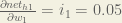
Putting it all together:

$\frac{\partial E_{total}}{\partial w_{1}} = \frac{\partial E_{total}}{\partial out_{h1}} * \frac{\partial out_{h1}}{\partial net_{h1}} * \frac{\partial net_{h1}}{\partial w_{1}}$

$\frac{\partial E_{total}}{\partial w_{1}} = 0.036350306 * 0.241300709 * 0.05 = 0.000438568$

You might also see this written as:

$\frac{\partial E_{total}}{\partial w_{1}} = (\sum\limits_{o}{\frac{\partial E_{total}}{\partial out_{o}} * \frac{\partial out_{o}}{\partial net_{o}} * \frac{\partial net_{o}}{\partial out_{h1}}}) * \frac{\partial out_{h1}}{\partial net_{h1}} * \frac{\partial net_{h1}}{\partial w_{1}}$

$\frac{\partial E_{total}}{\partial w_{1}} = (\sum\limits_{o}{\delta_{o} * w_{ho}}) * out_{h1}(1 - out_{h1}) * i_{1}$

$\frac{\partial E_{total}}{\partial w_{1}} = \delta_{h1}i_{1}$

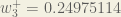
We can now update $w_1$ :

$w_1^{+} = w_1 - \eta * \frac{\partial E_{total}}{\partial w_{1}} = 0.15 - 0.5 * 0.000438568 = 0.149780716$

Repeating this for $w_2$ , $w_3$ , and $w_4$

$w_2^{+} = 0.19956143$

$w_3^{+} = 0.24975114$

$w_4^{+} = 0.29950229$

Finally, we’ve updated all of our weights! When we fed forward the 0.05 and 0.1 inputs originally, the error on the network was 0.298371109. After this first round of backpropagation, the total error is now down to 0.291027924. It might not seem like much, but after repeating this process 10,000 times, for example, the error plummets to 0.0000351085. At this point, when we feed forward 0.05 and 0.1, the two outputs neurons generate 0.015912196 (vs 0.01 target) and 0.984065734 (vs 0.99 target).

If you’ve made it this far and found any errors in any of the above or can think of any ways to make it clearer for future readers, don’t hesitate to drop me a note. Thanks!

And while I have you…

Again, if you liked this tutorial, please check out Emergent Mind, a site I’m building with an end goal of explaining AI/ML concepts in a similar style as this post. Feedback very much welcome!

1,111 thoughts on “A Step by Step Backpropagation Example”

Hari Prasad says:

September 12, 2016 at 4:51 am

This is how any teaching or learning has to happen! Great work buddy!

Reply
rambo says:

September 12, 2016 at 6:22 pm

Many thanks. The best tutorial I have ever seen

Reply
Erhard M. Dinhobl says:

September 13, 2016 at 7:30 am

It seems that the learningrate of “0.5” in this example here is too high. because it diverges with the given values. Maybe 0.05?

Reply
1. Erhard M. Dinhobl says:
  
  September 13, 2016 at 10:39 am
  
  sorry, forgot to set the energy variable in the neuron back to zero after training
  
  Reply
Michael Prager says:

September 17, 2016 at 7:17 pm

I found this post very helpful but there is one thing that is confusing me. You apply the logistic function on the output nodes to compute out_o1 and out_o2 as the sigmoid function applied to the weighted sum of the hidden nodes. My question is, what if you are predicting an output that has a range wider than 0 to 1. I had thought the output layer was simply a weighted sum of the outputs of the final hidden layer. In that case you could output a value in any range, but this seems very limiting.

Reply
1. Mazur says:
  
  September 18, 2016 at 10:39 am
  
  Yeah, this only works on a range of 0 to 1. If you have a range from say 0 to 100 you can divide by 100 to get it down to a range of 0 to 1 so that you can use this neural network.
  
  Reply
Gregory says:

September 20, 2016 at 2:20 am

what does the Who mean in the expression for the hidden layers?
The “ho” is small

Reply
1. Mazur says:
  
  September 20, 2016 at 8:19 pm
  
  Weight of the hidden output.
  
  Reply
  1. Gregory says:
    
    September 23, 2016 at 9:25 pm
    
    Shouldn’t it be the weights connecting the last hidden layer and the output layer? If the network had an input of 200, hidden of 100, and another hidden of 50, and an output of 10; it wouldn’t work. Because the layer of 1 hundred would add the outputs multiplied by 10 of the 50 layer weights, right? Sorry if I am not very clear. What I’m just trying to ask is this: Is the Who referring to the weight connecting the last layer and output layer or is it connecting the current layer and next layer?
    
    Reply
Anirban says:

September 20, 2016 at 3:27 am

You have used a squared error function. When using that as a cost function along with the sigmoid function, won’t your cost function have a lot of local minima ?

Reply
Hajji Hicham says:

September 20, 2016 at 6:55 am

Thanks, it’s the best and clear step by step tutorial of the backpropagation alg I have ever read

Reply
gsaldanha2 says:

September 21, 2016 at 12:37 am

Thanks so much!! It’s a very clear and thorough explanation :)

Reply
Roopak Neevan says:

September 21, 2016 at 1:17 am

Great Post with the step by step explanation.
Based on your explanation I am able to implement the same for LOGICAL GATE solution where I have used 2 Input Nodes (for logical Inputs), 1 Hidden Layer with 2 Nodes and one Output Node.
Thanks for this detailed explanation.
Regards
Neevan

Reply
Nimesh says:

September 22, 2016 at 2:44 am

Couldn’t agree less with Hajji.
Its one the best and simplified article.

Reply
research scholar says:

September 23, 2016 at 10:27 pm

Thanks for beautiful workout .algorithm has become transparent and very easy

Reply
Apoorva Bansal says:

September 25, 2016 at 12:52 am

Amazingly simple explanation to something everyone tends to complicate! :) Thanks a lot!!

Reply
H. Paudel says:

September 25, 2016 at 7:38 am

It was a great explanation, Mazur. Thank you very much for the effort.
It would be great if you could response my following query.
I have been trying to train a model using neuralnet package. My model contains five input one output and a hidden layer with 10 nodes. logistic transfer function is selected as an activation function. All data are normalized in 0,1 range. As the logistic function is bounded between 0,1 the results are expected to be in the range 0,1. But some of the training results are negative. What is causing the model to compute negative output?
Regards
H. Paudel

Reply
gsaldanha2 says:

September 25, 2016 at 11:40 pm

How would you compute the weight for a hidden layer in a multi-layer network?

Reply
Pingback: 反向传播算法入门资源索引 | 我爱自然语言处理
Pingback: Building a multi-class text classifier from scratch using Neural Networks – Stokastik
agusta says:

October 1, 2016 at 7:59 pm

you’re the saviour!

Reply
Lukas says:

October 4, 2016 at 4:15 am

Many thanks for tutorial!

But I have a problem, when im trying use more neurons (e.g. 20 inputs and 8 outputs) with more training data, NN total error is almost stagnates after few cycles. Any solution? (adaptive eta?)

Reply
1. Danilo says:
  
  October 28, 2016 at 12:55 am
  
  Convert your input data to decimal values between 0 and 1 only.
  
  Reply
satheesh Raja Raju says:

October 5, 2016 at 7:31 pm

Hi – Thanks much , this is the only place I got some valid information in a way I can understand. I have few questions, if you don’t can you please check these out.

Question 1:
You have tried to find derivative of Etotal WRT to W5.

In this how did you get this “-1”(Minus 1), doesn’t the derivate rule equate to following

2*1/2(targeto1-out01) ( No Minus)

Question 2:
In chain rule. To find derivative of Etotal WRT to W5 following was used.

DEtotal/Dw5 = Dnet01/Dw5 * Dout01/ Dnet01 * DEtotal/DOut01

Here please note : DOut01/Dnet01 , Out01 was used and It makes sense.

But to To find derivative of Etotal WRT to W1 following was used.

DOut01/Dnet01 was not used, why is that.

Reply
1. Hari Seshadri says:
  
  October 8, 2016 at 9:20 pm
  
  Question 1: Using chain rule, since out_01 has a negative sign before it in the parenthesis, you need to propagate (no pun intended) that negative sign. In other words:
  
  \frac{d}{dx} {(1-x)}^2 = (-1) \times (2-1) \times {(1-x)}^{(2-1)}
  
  Question 2:
  
  Check out the image beneath the writing “Next, we’ll continue the backwards pass by calculating new values for w1, w2, w3, and w4”. He explains that D(E_total)/D(out_h1) = D(E_o1)/D(Out_h1) + D(E_o2)/D(Out_h1). And then he breaks out that first term, D(E_o1)/D(Out_h1), in the next images, which includes your term “DOut01/Dnet01”
  
  Reply
  1. satheesh says:
    
    October 12, 2016 at 7:07 pm
    
    Hi Hari – Thank you for your patience and answer. May be I am missing something here, on question 1.
    
    Here derivate of E total WRT Out01 is (target01 – Out01), so the correct value is “-0.74136507”.
    
    Minus sign stating derivative in decreasing , going in downward direction.
    
    I am still not sure how “-0.74136507” changed to “0.74136507”
    
    Reply
    1. mkei says:
      
      November 1, 2016 at 7:29 pm
      
      I am also not sure where the * -1 comes from, there is not a multiplication there in the non-differentiated function. It seems odd.
      
      Reply
2. hariseshadri says:
  
  October 8, 2016 at 9:21 pm
  
  Question 1: Using chain rule, since out_01 has a negative sign before it in the parenthesis, you need to propagate (no pun intended) that negative sign. In other words:
  
  \frac{d}{dx} {(1-x)}^2 = (-1) \times (2-1) \times {(1-x)}^{(2-1)}
  
  Question 2:
  
  Check out the image beneath the writing “Next, we’ll continue the backwards pass by calculating new values for w1, w2, w3, and w4”. He explains that D(E_total)/D(out_h1) = D(E_o1)/D(Out_h1) + D(E_o2)/D(Out_h1). And then he breaks out that first term, D(E_o1)/D(Out_h1), in the next images, which includes your term “DOut01/Dnet01”
  
  Reply
3. Larry Smith says:
  
  May 28, 2017 at 9:19 am
  
  See this explanation https://www.symbolab.com/solver/derivative-calculator/%5Cfrac%7B%5Cpartial%20%7D%7B%5Cpartial%20%20x%7D%5Cleft(%5Cleft(1-x%5Cright)%5E%7B2%7D%5Cright)
  
  Reply
Giovanni says:

October 10, 2016 at 6:10 am

Mazur, Thank you for your explanation, but i have a little question, i have calculated exactly the same steps you described, but the second round i calculated the total error is 0.292165448
different from what you have written, i have done something wrong in your opinion?

Reply
Huy says:

October 14, 2016 at 4:20 pm

I have a small question. From your tutorial, the node delta is calculated as
(out – target) * out (1 – out)
I tried implementing the XOR network here:
http://www.heatonresearch.com/aifh/vol3/xor_batch.html
and it fails to find the optimal weights. It turns out that the node delta in the above website is
(target – out) * out (1 – out)
Why is there a sign difference?
Thanks so much!

Reply
Pingback: 神经网络101 手把手快速入门神经网络基础 | David 9的博客 --- 没有"过拟合"
chuckwolber says:

October 16, 2016 at 3:30 pm

If you read the original 1986 paper (Learning representations by back-propagating errors), you will find that they calculate the error function in the reverse (out – target). I believe the math works out the same, but the general consensus from a variety of sources is to calculate it as -(target – out).

I would be curious what the original authors, or even Yann LeCun, has to say about this.

You allude to this curiosity early in your rundown. I figured it would be worthwhile to point out its potential origin.

Reply
Couhp says:

October 19, 2016 at 11:50 pm

Thank you =))))

Reply
markpppp says:

October 21, 2016 at 6:03 am

I cannot thank you enough!

Reply
Alex says:

October 22, 2016 at 3:35 pm

Thank you very much for a great lesson.
When I calculate the first forward pass i get the same output, same total error and the same value for the new weights as in your example.

But when I run a second time I get 0,291027774 instead of 0,291027924.

After 10000 turns i get 3,5109E-05 instead of 3,5085E-05
I use double as datatype and do not round the values

Reply
wxfeng says:

October 23, 2016 at 7:09 pm

Reblogged this on Site Title.

Reply
Jack says:

October 24, 2016 at 10:25 pm

This article is amazing and really helped me to understand backwards propagation! Very well-written and intuitive to follow. As a test, I tried transposing your Python code into Swift. I tested all your inputs/outputs to my program and it outputted the same numbers (save for some *very* negligible differences), so I believe it’s constructed correctly. Even when testing your very last paragraph (inputs: 0.05, 0.1, expected outputs: 0.01, 0.99, backwards propagated 10,000 times) it ended up with the same output. However, I’m having some trouble training it to do other things.

To play with it, I decided to train it with OR operator testing inputs. I gave it two input neurons, five hidden neurons, and one output neuron. The tests were:

network.train(inputs: [0,0], expectedOutputs: [0])
network.train(inputs: [0,1], expectedOutputs: [1])
network.train(inputs: [1,0], expectedOutputs: [1])
network.train(inputs: [1,1], expectedOutputs: [0])

And I had the program repeat these 4 lines of code 10,000 times. At the end, when I forward propagated it, all the outputs were about 0.5 (making the error margin approximately 0.5) and it the outputs barely changed since the beginning! What’s up with this? Am I not training it correctly, or would something be wrong with my code? I can upload the source if that will help.

Thank you so much to whoever can help.

Reply
1. Huy says:
  
  October 26, 2016 at 9:37 pm
  
  Hi,
  I had the same issue. I believe that the node delta has the wrong sign. It should be (target – out) instead of -(target – out).
  If you change the sign then it should work. Here’s another useful website for checking your calculations:
  
  http://www.heatonresearch.com/aifh/vol3/xor_batch.html
  
  If you build a similar XOR network, every time you click “Train batch epoch” the web build display all relevant calculations.
  
  Once you switch the sign, all logical operators work. :D
  
  Reply
formybaby2016 says:

October 25, 2016 at 11:11 am

Please help me to answer this question. I’m confusing with calculation partial derivative of Eo2 with respect outo1 (dE02/dOut01).
You wrote: “Following the same process for dE02/dOut01, we get: dE02/dOuth1=-0.019049119”
E02 = 1/2(target02 – out02)^2, therefore the partial derivative of E02 with respect out01 will be 0. So how can you get
dE02/dOuth1=-0.019049119?
Thank you in advance!

Reply
Joe says:

October 26, 2016 at 10:12 pm

I’ve bookmarked this and have come back so many times I just have to let you know how awesome it is.

Reply
Kamil says:

October 28, 2016 at 3:42 pm

Can someone PLEASE explain to me how this got calculated?
https://s0.wp.com/latex.php?latex=%5Cfrac%7B%5Cpartial+E_%7Btotal%7D%7D%7B%5Cpartial+out_%7Bo1%7D%7D+%3D+2+%2A+%5Cfrac%7B1%7D%7B2%7D%28target_%7Bo1%7D+-+out_%7Bo1%7D%29%5E%7B2+-+1%7D+%2A+-1+%2B+0&bg=ffffff&fg=404040&s=0

Reply
1. Kamil says:
  
  October 31, 2016 at 4:41 pm
  
  Ok I got it
  
  Reply
Garima says:

October 30, 2016 at 2:18 am

Your explanation is very nice sir. I think you can add little more derivation. Likr after applying the penalty term (theta exponent T theta)to error function what wil be the derivation

Reply
Kamil says:

October 31, 2016 at 4:41 pm

Why is dError/dHidden1 calculated without including the net_o1 and out_o1?

Reply
xxoospring says:

November 1, 2016 at 10:12 pm

nice blog! hope for next addition can related this algorithm to coding(Python,c
++) or show how the vectorization works

Reply
Pingback: Best articles to learn deep learning | Learn for Master
Query says:

November 6, 2016 at 5:29 am

When you calculate neth1 shouldn’t you be multiplying 0.25 with 0.1 instead of 0.2?

Reply
Query says:

November 6, 2016 at 5:36 am

Similarly for neto1, you should be multiplying w7 with out h2 because that is the input of o1 instead of w6.

Reply
Pankaj Rawat says:

November 10, 2016 at 7:41 am

The most clear explanation of back propagation i have come across.

Reply
Pingback: David Asboth | Data and Software | Why You Should Reinvent the Machine Learning Wheel
mohan chakradhar says:

November 12, 2016 at 1:08 pm

Wow…very simple explanation for such a complicated process…

Thanks

Reply
Niloufar says:

November 12, 2016 at 2:30 pm

thank you very much
it was so good :D

Reply
Caspar says:

November 13, 2016 at 7:28 am

Really great tutorial. How would the pattern of back propagation carry on with multiple hidden layers instead of just the one? What would the overall algorithm look like where the hidden layer count, weights, etc, are all variable?

Reply
1. Shakezz says:
  
  January 27, 2017 at 5:54 pm
  
  I also would be very interested in the answer!
  
  Reply
Raphael Guimarães says:

November 15, 2016 at 8:01 pm

OMG you saved my life!

Reply
Lukas Cerny says:

November 16, 2016 at 5:18 am

Thank you an amazing article! Everywhere else the description of the algorithm is extremely theoretically, so I am glad that you got your hands dirty by really describing the actual implementation with numbers and not just by loads of symbols, which particularly in the case of backpropagation was very confusing for me. Cheers from Edinburgh.

Reply
Caspar says:

November 16, 2016 at 9:46 am

Having a read now – seems really helpful. Thank you!

Reply
1. shyamkkhadka says:
  
  December 10, 2016 at 12:16 pm
  
  Hello Caspar, did you get information about how to implement it for multiple hidden layer ? I am also looking for this. Thank you.
  
  Reply
  1. Sandip Dhakal says:
    
    January 23, 2017 at 2:02 pm
    
    https://github.com/jovianlin/siraj-intro-to-DL-02/blob/master/MultiLayerNeuralNetwork.ipynb
    
    Reply
Vadym says:

November 17, 2016 at 9:45 pm

Thanks for great article!
Question: how do we tune the weights of biases?

Reply
1. George Pligoropoulos says:
  
  December 22, 2016 at 7:26 am
  
  Yes how do we find the updated biases??
  
  Reply
  1. Mehrdad says:
    
    January 16, 2017 at 7:27 am
    
    Hi there,
    I think those are same with same layer’s weight but the output value won’t update.( in example suppose 1 for biases weight )
    
    Reply
    1. Mehrdad says:
      
      January 16, 2017 at 7:32 am
      
      Sorry Matt please update my post with this:
      Hi there,
      I think those are same with same layer’s weight but the value of biases won’t update.( in example supposed 1 for biases weight )
      
      Reply
Viral Parekh says:

November 18, 2016 at 12:51 pm

Nicely explained ! :) Thank you.

Reply
Pingback: Exploring Neural Networks… – Cluster Chord
ali hesri says:

November 20, 2016 at 2:51 pm

great

Reply
Syed says:

November 20, 2016 at 2:54 pm

Thanks alot for such a wonderful explanation.

Reply