A Step by Step Backpropagation Example

March 17, 2015February 23, 2024Mazur

Background

Backpropagation is a common method for training a neural network. There is no shortage of papers online that attempt to explain how backpropagation works, but few that include an example with actual numbers. This post is my attempt to explain how it works with a concrete example that folks can compare their own calculations to in order to ensure they understand backpropagation correctly.

Backpropagation in Python

You can play around with a Python script that I wrote that implements the backpropagation algorithm in this Github repo.

Continue learning with Emergent Mind

If you find this tutorial useful and want to continue learning about AI/ML, I encourage you to check out Emergent Mind, a new website I’m working on that uses GPT-4 to surface and explain cutting-edge AI/ML papers:

In time, I hope to use AI to explain complex AI/ML topics on Emergent Mind in a style similar to what you’ll find in the tutorial below.

Now, on with the backpropagation tutorial…

Overview

For this tutorial, we’re going to use a neural network with two inputs, two hidden neurons, two output neurons. Additionally, the hidden and output neurons will include a bias.

Here’s the basic structure:

In order to have some numbers to work with, here are the initial weights, the biases, and training inputs/outputs:

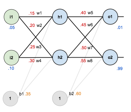
The goal of backpropagation is to optimize the weights so that the neural network can learn how to correctly map arbitrary inputs to outputs.

For the rest of this tutorial we’re going to work with a single training set: given inputs 0.05 and 0.10, we want the neural network to output 0.01 and 0.99.

The Forward Pass

To begin, lets see what the neural network currently predicts given the weights and biases above and inputs of 0.05 and 0.10. To do this we’ll feed those inputs forward though the network.

We figure out the total net input to each hidden layer neuron, squash the total net input using an activation function (here we use the logistic function), then repeat the process with the output layer neurons.

Total net input is also referred to as just net input by some sources.

Here’s how we calculate the total net input for $h_1$ :

$net_{h1} = w_1 * i_1 + w_2 * i_2 + b_1 * 1$

$net_{h1} = 0.15 * 0.05 + 0.2 * 0.1 + 0.35 * 1 = 0.3775$

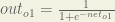
We then squash it using the logistic function to get the output of $h_1$ :

$out_{h1} = \frac{1}{1+e^{-net_{h1}}} = \frac{1}{1+e^{-0.3775}} = 0.593269992$

Carrying out the same process for $h_2$ we get:

$out_{h2} = 0.596884378$

We repeat this process for the output layer neurons, using the output from the hidden layer neurons as inputs.

Here’s the output for $o_1$ :

$net_{o1} = w_5 * out_{h1} + w_6 * out_{h2} + b_2 * 1$

$net_{o1} = 0.4 * 0.593269992 + 0.45 * 0.596884378 + 0.6 * 1 = 1.105905967$

$out_{o1} = \frac{1}{1+e^{-net_{o1}}} = \frac{1}{1+e^{-1.105905967}} = 0.75136507$

And carrying out the same process for $o_2$ we get:

$out_{o2} = 0.772928465$

Calculating the Total Error

We can now calculate the error for each output neuron using the squared error function and sum them to get the total error:

$E_{total} = \sum \frac{1}{2}(target - output)^{2}$

Some sources refer to the target as the ideal and the output as the actual.

The $\frac{1}{2}$ is included so that exponent is cancelled when we differentiate later on. The result is eventually multiplied by a learning rate anyway so it doesn’t matter that we introduce a constant here [1].

For example, the target output for $o_1$ is 0.01 but the neural network output 0.75136507, therefore its error is:

$E_{o1} = \frac{1}{2}(target_{o1} - out_{o1})^{2} = \frac{1}{2}(0.01 - 0.75136507)^{2} = 0.274811083$

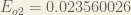
Repeating this process for $o_2$ (remembering that the target is 0.99) we get:

$E_{o2} = 0.023560026$

The total error for the neural network is the sum of these errors:

$E_{total} = E_{o1} + E_{o2} = 0.274811083 + 0.023560026 = 0.298371109$

The Backwards Pass

Our goal with backpropagation is to update each of the weights in the network so that they cause the actual output to be closer the target output, thereby minimizing the error for each output neuron and the network as a whole.

Output Layer

Consider $w_5$ . We want to know how much a change in $w_5$ affects the total error, aka $\frac{\partial E_{total}}{\partial w_{5}}$ .

$\frac{\partial E_{total}}{\partial w_{5}}$ is read as “the partial derivative of $E_{total}$ with respect to $w_{5}$ “. You can also say “the gradient with respect to $w_{5}$ ”.

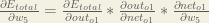
By applying the chain rule we know that:

$\frac{\partial E_{total}}{\partial w_{5}} = \frac{\partial E_{total}}{\partial out_{o1}} * \frac{\partial out_{o1}}{\partial net_{o1}} * \frac{\partial net_{o1}}{\partial w_{5}}$

Visually, here’s what we’re doing:

We need to figure out each piece in this equation.

First, how much does the total error change with respect to the output?

$E_{total} = \frac{1}{2}(target_{o1} - out_{o1})^{2} + \frac{1}{2}(target_{o2} - out_{o2})^{2}$

$\frac{\partial E_{total}}{\partial out_{o1}} = 2 * \frac{1}{2}(target_{o1} - out_{o1})^{2 - 1} * -1 + 0$

$\frac{\partial E_{total}}{\partial out_{o1}} = -(target_{o1} - out_{o1}) = -(0.01 - 0.75136507) = 0.74136507$

$-(target - out)$ is sometimes expressed as $out - target$

When we take the partial derivative of the total error with respect to $out_{o1}$ , the quantity $\frac{1}{2}(target_{o2} - out_{o2})^{2}$ becomes zero because $out_{o1}$ does not affect it which means we’re taking the derivative of a constant which is zero.

Next, how much does the output of $o_1$ change with respect to its total net input?

The partial derivative of the logistic function is the output multiplied by 1 minus the output:

$out_{o1} = \frac{1}{1+e^{-net_{o1}}}$

$\frac{\partial out_{o1}}{\partial net_{o1}} = out_{o1}(1 - out_{o1}) = 0.75136507(1 - 0.75136507) = 0.186815602$

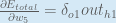
Finally, how much does the total net input of $o1$ change with respect to $w_5$ ?

$net_{o1} = w_5 * out_{h1} + w_6 * out_{h2} + b_2 * 1$

$\frac{\partial net_{o1}}{\partial w_{5}} = 1 * out_{h1} * w_5^{(1 - 1)} + 0 + 0 = out_{h1} = 0.593269992$

Putting it all together:

$\frac{\partial E_{total}}{\partial w_{5}} = \frac{\partial E_{total}}{\partial out_{o1}} * \frac{\partial out_{o1}}{\partial net_{o1}} * \frac{\partial net_{o1}}{\partial w_{5}}$

$\frac{\partial E_{total}}{\partial w_{5}} = 0.74136507 * 0.186815602 * 0.593269992 = 0.082167041$

You’ll often see this calculation combined in the form of the delta rule:

$\frac{\partial E_{total}}{\partial w_{5}} = -(target_{o1} - out_{o1}) * out_{o1}(1 - out_{o1}) * out_{h1}$

Alternatively, we have $\frac{\partial E_{total}}{\partial out_{o1}}$ and $\frac{\partial out_{o1}}{\partial net_{o1}}$ which can be written as $\frac{\partial E_{total}}{\partial net_{o1}}$ , aka $\delta_{o1}$ (the Greek letter delta) aka the node delta. We can use this to rewrite the calculation above:

$\delta_{o1} = \frac{\partial E_{total}}{\partial out_{o1}} * \frac{\partial out_{o1}}{\partial net_{o1}} = \frac{\partial E_{total}}{\partial net_{o1}}$

$\delta_{o1} = -(target_{o1} - out_{o1}) * out_{o1}(1 - out_{o1})$

Therefore:

$\frac{\partial E_{total}}{\partial w_{5}} = \delta_{o1} out_{h1}$

Some sources extract the negative sign from $\delta$ so it would be written as:

$\frac{\partial E_{total}}{\partial w_{5}} = -\delta_{o1} out_{h1}$

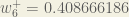
To decrease the error, we then subtract this value from the current weight (optionally multiplied by some learning rate, eta, which we’ll set to 0.5):

$w_5^{+} = w_5 - \eta * \frac{\partial E_{total}}{\partial w_{5}} = 0.4 - 0.5 * 0.082167041 = 0.35891648$

Some sources use $\alpha$ (alpha) to represent the learning rate, others use $\eta$ (eta), and others even use $\epsilon$ (epsilon).

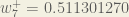
We can repeat this process to get the new weights $w_6$ , $w_7$ , and $w_8$ :

$w_6^{+} = 0.408666186$

$w_7^{+} = 0.511301270$

$w_8^{+} = 0.561370121$

We perform the actual updates in the neural network after we have the new weights leading into the hidden layer neurons (ie, we use the original weights, not the updated weights, when we continue the backpropagation algorithm below).

Hidden Layer

Next, we’ll continue the backwards pass by calculating new values for $w_1$ , $w_2$ , $w_3$ , and $w_4$ .

Big picture, here’s what we need to figure out:

$\frac{\partial E_{total}}{\partial w_{1}} = \frac{\partial E_{total}}{\partial out_{h1}} * \frac{\partial out_{h1}}{\partial net_{h1}} * \frac{\partial net_{h1}}{\partial w_{1}}$

Visually:

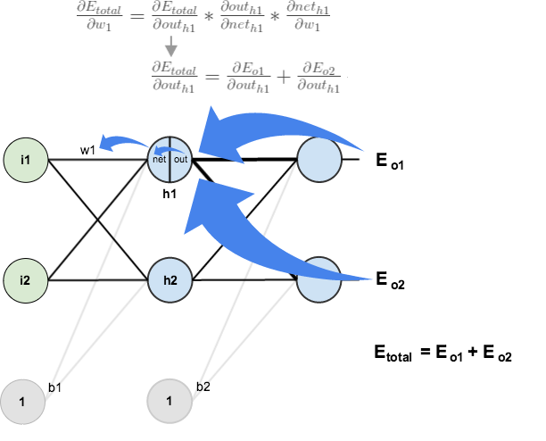
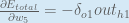
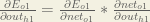
We’re going to use a similar process as we did for the output layer, but slightly different to account for the fact that the output of each hidden layer neuron contributes to the output (and therefore error) of multiple output neurons. We know that $out_{h1}$ affects both $out_{o1}$ and $out_{o2}$ therefore the $\frac{\partial E_{total}}{\partial out_{h1}}$ needs to take into consideration its effect on the both output neurons:

$\frac{\partial E_{total}}{\partial out_{h1}} = \frac{\partial E_{o1}}{\partial out_{h1}} + \frac{\partial E_{o2}}{\partial out_{h1}}$

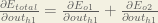
Starting with $\frac{\partial E_{o1}}{\partial out_{h1}}$ :

$\frac{\partial E_{o1}}{\partial out_{h1}} = \frac{\partial E_{o1}}{\partial net_{o1}} * \frac{\partial net_{o1}}{\partial out_{h1}}$

We can calculate $\frac{\partial E_{o1}}{\partial net_{o1}}$ using values we calculated earlier:

$\frac{\partial E_{o1}}{\partial net_{o1}} = \frac{\partial E_{o1}}{\partial out_{o1}} * \frac{\partial out_{o1}}{\partial net_{o1}} = 0.74136507 * 0.186815602 = 0.138498562$

And $\frac{\partial net_{o1}}{\partial out_{h1}}$ is equal to $w_5$ :

$net_{o1} = w_5 * out_{h1} + w_6 * out_{h2} + b_2 * 1$

$\frac{\partial net_{o1}}{\partial out_{h1}} = w_5 = 0.40$

Plugging them in:

$\frac{\partial E_{o1}}{\partial out_{h1}} = \frac{\partial E_{o1}}{\partial net_{o1}} * \frac{\partial net_{o1}}{\partial out_{h1}} = 0.138498562 * 0.40 = 0.055399425$

Following the same process for $\frac{\partial E_{o2}}{\partial out_{h1}}$ , we get:

$\frac{\partial E_{o2}}{\partial out_{h1}} = -0.019049119$

Therefore:

$\frac{\partial E_{total}}{\partial out_{h1}} = \frac{\partial E_{o1}}{\partial out_{h1}} + \frac{\partial E_{o2}}{\partial out_{h1}} = 0.055399425 + -0.019049119 = 0.036350306$

Now that we have $\frac{\partial E_{total}}{\partial out_{h1}}$ , we need to figure out $\frac{\partial out_{h1}}{\partial net_{h1}}$ and then $\frac{\partial net_{h1}}{\partial w}$ for each weight:

$out_{h1} = \frac{1}{1+e^{-net_{h1}}}$

$\frac{\partial out_{h1}}{\partial net_{h1}} = out_{h1}(1 - out_{h1}) = 0.59326999(1 - 0.59326999 ) = 0.241300709$

We calculate the partial derivative of the total net input to $h_1$ with respect to $w_1$ the same as we did for the output neuron:

$net_{h1} = w_1 * i_1 + w_3 * i_2 + b_1 * 1$

$\frac{\partial net_{h1}}{\partial w_1} = i_1 = 0.05$

Putting it all together:

$\frac{\partial E_{total}}{\partial w_{1}} = \frac{\partial E_{total}}{\partial out_{h1}} * \frac{\partial out_{h1}}{\partial net_{h1}} * \frac{\partial net_{h1}}{\partial w_{1}}$

$\frac{\partial E_{total}}{\partial w_{1}} = 0.036350306 * 0.241300709 * 0.05 = 0.000438568$

You might also see this written as:

$\frac{\partial E_{total}}{\partial w_{1}} = (\sum\limits_{o}{\frac{\partial E_{total}}{\partial out_{o}} * \frac{\partial out_{o}}{\partial net_{o}} * \frac{\partial net_{o}}{\partial out_{h1}}}) * \frac{\partial out_{h1}}{\partial net_{h1}} * \frac{\partial net_{h1}}{\partial w_{1}}$

$\frac{\partial E_{total}}{\partial w_{1}} = (\sum\limits_{o}{\delta_{o} * w_{ho}}) * out_{h1}(1 - out_{h1}) * i_{1}$

$\frac{\partial E_{total}}{\partial w_{1}} = \delta_{h1}i_{1}$

We can now update $w_1$ :

$w_1^{+} = w_1 - \eta * \frac{\partial E_{total}}{\partial w_{1}} = 0.15 - 0.5 * 0.000438568 = 0.149780716$

Repeating this for $w_2$ , $w_3$ , and $w_4$

$w_2^{+} = 0.19956143$

$w_3^{+} = 0.24975114$

$w_4^{+} = 0.29950229$

Finally, we’ve updated all of our weights! When we fed forward the 0.05 and 0.1 inputs originally, the error on the network was 0.298371109. After this first round of backpropagation, the total error is now down to 0.291027924. It might not seem like much, but after repeating this process 10,000 times, for example, the error plummets to 0.0000351085. At this point, when we feed forward 0.05 and 0.1, the two outputs neurons generate 0.015912196 (vs 0.01 target) and 0.984065734 (vs 0.99 target).

If you’ve made it this far and found any errors in any of the above or can think of any ways to make it clearer for future readers, don’t hesitate to drop me a note. Thanks!

And while I have you…

Again, if you liked this tutorial, please check out Emergent Mind, a site I’m building with an end goal of explaining AI/ML concepts in a similar style as this post. Feedback very much welcome!

1,112 thoughts on “A Step by Step Backpropagation Example”

Nitzan Wilnai says:

April 27, 2017 at 6:49 pm

This is really great. Like the others I have 2 questions. Why aren’t you updating the bias weights, and when moving to w1-w4, should we use the original w5-w8 or the new updated ones?

Reply
DADI says:

April 28, 2017 at 10:47 am

Thanks for this article….But i would like to know how performing backpropagation using deep learning? if you can give me an example of how training a DB of n 2D images.

Reply
TOMAZ STIH says:

April 29, 2017 at 10:07 am

Great work. I was able to develop my first net using your tutorial as a test case. One question: using Etotal one can update weights for the output layer. Then using both E1 and E2 one can update weights for the hidden layer. What would you use for errors if you had more then one hidden layer (same E1 and E2?)

Reply
Joshua Laferriere says:

April 30, 2017 at 2:35 am

spreadsheet implementation, messy but the #’s work

https://docs.google.com/spreadsheets/d/1ashrhJsLaCgusiJM2n_Y-zB5Usshxp9jIrNJbf-_vwU/edit?usp=sharing

Reply
1. jseprofits says:
  
  June 24, 2017 at 3:50 pm
  
  Messy but brilliant. Was about to do it in Excel so you saved me a weekend. Thank you. Well done.
  
  Reply
Nattapat Attiratanasunthron says:

May 2, 2017 at 2:40 am

thank you very much for best example

Reply
Kumar Deepankar says:

May 3, 2017 at 1:14 am

Wow. could not ask for much granular level explanation. Thanks so much.

Reply
M Karthikeyan says:

May 3, 2017 at 10:42 am

Thanks for this useful explanation. I have a doubt if you have the time. Can the same back propagation be modified slightly to work with a convolution neural net. Any comments would be very helpful.

Reply
1. MsMC says:
  
  June 21, 2017 at 12:09 pm
  
  At the start of backward propgation, why is the E_total being considered for partial derivative with respect to w5. Shouldn’t it just be E_01? (Since E_02 doesn’t have any effect of changing w5).
  
  Reply
Satya says:

May 4, 2017 at 8:12 am

Matt good explanation. One quick question is that you pointed out after 10k iteration the error should drop. Does that mean to repeat with same instance (ie i1 is 0.05 and i2 is 0.10) or do you randomly generate i1=2*i2 where 0<i1<0.45 of 10k instances

Reply
Suchir Bhatnagar says:

May 5, 2017 at 2:08 am

Hi,
While calculating H1 should we not use the weight 0.25 and not 0.20

Reply
1. matze says:
  
  June 17, 2017 at 12:33 pm
  
  Nope, I had the same issue, but the sketch of the net is a little bit confusing.
  
  Reply
Abdul Waheed says:

May 5, 2017 at 2:24 am

“Maa Shaa Allah”, Great Skills. First time i understood completely what is Back propagation. I am PhD student @ bsauniv.ac.in

Reply
raghu says:

May 5, 2017 at 3:47 am

At the end I have understood backpropagation. Thank you

Reply
bob sam says:

May 5, 2017 at 7:50 am

Thanks to your simple explanation of backpropagation I was able to successfully build a neural network in java. You have the best explanation of this stuff on the internet!

Reply
Aram says:

May 5, 2017 at 8:34 am

Sir, first of all, it is very clear. However; I think you should use the updated weights for the next training input not the same input.
Can you kindly clarify that?

Reply
Pingback: 反向传播算法入门资源索引 | 机器虫
Sushant says:

May 9, 2017 at 1:03 am

Thanks Matt. This is very helpful. I a newbie question. How that the NN is trained how can i use this code to give me an output of 0.01,0.99 when the input is 0.05,0.1

Reply
dataminor says:

May 10, 2017 at 5:15 am

it is cool! thx!

Reply
Ryan says:

May 14, 2017 at 12:03 pm

What are the weights after the 10,000 iteration?

Reply
Fernando says:

May 15, 2017 at 8:06 pm

Hi, first I´d like to thank you. this tutorial made everything clear to me and helped me building my neural network.
But, I have a question, What book or referencee did you use to learn to develope this tutorial ? I really liked the way you exposed the topic, so I wanted to learn a little bit more.

Hoping for hearing from you soon.

Reply
emoron says:

May 17, 2017 at 11:58 am

Reblogged this on Diplomado La Ciencia en tu Escuela.

Reply
Mohamed Abd Elhamid says:

May 17, 2017 at 9:09 pm

great work , thanks

Reply
Maashu says:

May 20, 2017 at 8:31 am

This truly is an amazing explanation of backpropogation!

I’m stuck on one thing though, and I could really use some help. Just after this statement:

>>First, how much does the total error change with respect to the output?

There’s a negative one (-1) in the formula of the partial derivative that I can’t for the life of me figure out where it’s coming from.

Any help is greatly appreciated, thanks so much!

Reply
1. Timothy Kanarsky says:
  
  June 12, 2017 at 8:52 am
  
  A bit late, but hope this helps:
  
  The -1 is a result of the chain rule. Let target[o1] be x and out[o1] be y. Then the expression we want to differentiate (ignoring the output and target of o2) is (1/2)*(x – y)^2. We first find the derivative of the outer expression (using the power rule): 2*(1/2)*(x – y), which simplifies to (x – y). We need to continue differentiating, however, because x is constant and does not vary with y. So the derivative of -y is -1. Then, by the chain rule, we multiply the derivatives of inner and outer expressions: (x-y)*-1. That’s where the -1 comes from! Hope this helps!
  
  Reply
  1. elchroy says:
    
    June 14, 2017 at 5:38 am
    
    I had this confusion too. Thanks for clarifying.
    
    Reply
  2. Matthew says:
    
    June 19, 2017 at 5:34 pm
    
    Yes, perfect, thanks so much!
    
    Reply
  3. maashu says:
    
    June 19, 2017 at 5:35 pm
    
    Yes, thanks so much!
    
    Reply
Farid Haziyev says:

May 21, 2017 at 5:26 pm

Thank you so much. It was very helpful and clear.

Reply
Mike W says:

May 31, 2017 at 9:00 am

Thanks much – this is very helpful. But one question: Shouldn’t the b1 and b2 values also get updated during the back propagation? Or did I miss that?

Reply
Pingback: LSTMs in even more excruciating detail – statisticalinterference
Leo says:

June 1, 2017 at 8:23 pm

Thanks a lot. You clearly explained everything.

Reply
John says:

June 4, 2017 at 12:48 am

Thanks so much. Finally I understand backprop.

Reply
Yuumnam Kirani Singh says:

June 7, 2017 at 4:36 am

Nice tutorial, well explained!

Reply
Breezy says:

June 11, 2017 at 3:15 pm

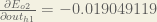
In backpropagation how is E_o2/out_h1 = -0.019049119 is calculated? What is the chain rule equation for this? i am not getting how to relate error E_02 and h_1. Kindly help me

Reply
1. Björn Ahlqvist says:
  
  June 23, 2017 at 4:55 pm
  
  I’m getting -0.0171442..
  
  Reply
rudiar7a says:

June 15, 2017 at 2:36 am

your the man brooo thanks ….

Reply
rudiar7a says:

June 15, 2017 at 2:37 am

Reblogged this on ARTA Story.

Reply
Minh says:

June 15, 2017 at 2:56 am

Very good example, thank you very much!

Reply
toancadet says:

June 16, 2017 at 2:26 pm

It is very detail of Backpropagation NN, Thanks!

and, I has a question to more detail:
In this example, you had only one pattern {0.5, 0.1}, so you repeated the training many times on the pattern. If I have a patterns vector (many pattern to input), then at each repeating, we will use next pattern (of the vector)?

one more, Thanks!

Reply
Sean Walton says:

June 16, 2017 at 3:27 pm

I want to be able to create a neural net that can recognize voiced phonemes. This means that I will not know how many A-to-D samples I will get until the pattern completes. I guess a network could check sample by sample, returning a FAIL, until the phoneme finishes. Do you have any ideas?

Reply
Jacob Johnson says:

June 16, 2017 at 4:37 pm

Where you’re calculating the derivative of netO1 with respect to w5, you’re taking w5 to the power of (1-1) which should be to the power of 0, which should be equal to just 1. Instead, you put .59 (the value of w5) there. What gives?

Reply
LuiGy Machaca says:

June 20, 2017 at 1:04 pm

Nice tutorial, well explained!

Reply
Subramanyam Natarajan says:

June 20, 2017 at 8:04 pm

Thanks a ton!!

Reply
ThangPM says:

June 21, 2017 at 2:20 am

Thank you so much for your post!!! I really appreciate it!

Reply
Pingback: Homer Simpson Guide to Backpropagation | Sefik Ilkin Serengil
jseprofits says:

June 24, 2017 at 3:46 pm

Matt
I am very new to ML but I am ok with Math. Thank so much for a very good illustration. Made so much more sense to me. To many tutorials remove the rigorous treatment you put in.
Thank you.
Mike, Cape Town, South Africa
Ps: Have you thought of doing this with an Excel as well?

Reply
zeycus says:

June 27, 2017 at 4:38 am

Thank you! This help me find a mistake in my neural network implementation. I added a unittest making sure a backpropagation step produces just these outputs.

Reply
Julia says:

June 28, 2017 at 9:27 pm

Thank you very much! It helps a lot! Very useful article!

Reply
Anuj Sharma says:

June 30, 2017 at 2:24 am

what is the use of bias in neural networks?
it would be great Matt sir if you elaborate my doubt with another brilliant example.

Reply
1. Mehrdad says:
  
  July 26, 2017 at 4:10 pm
  
  Hi Anuj,
  With my experience, I find 2 reasons for use bias. before explain those let me say bias it not useful to all network we design.
  reason 1: If you look at bias you see that bias doesn’t contact with inputs and just update with other weights because of this biasses make such a momentum in the network and help network doesn’t stick in very small local minimums.
  reason 2: In some cases, bias can help to ignore such a calculation errors, by that I mean for instance you have less chance to have sig( sum=0 ). I should say that again I have some network that doesn’t have any bias.
  
  Reply
Ravi Shankar says:

June 30, 2017 at 6:52 am

Nice supplement especially for a beginnner who has started with Andrew Ng course. Example makes it clear. Thank you

Reply
1. Mario Scalas says:
  
  August 20, 2017 at 3:37 pm
  
  Are you also stuck while computing the backpropagation derivatives? :D (Yeah, following Andrew Ng course too ;))
  
  Reply
Phimmasone says:

July 3, 2017 at 10:30 am

It is very useful ever for me, thank you so much.

Reply
Rishab says:

July 8, 2017 at 9:23 am

Hey, thanks for the clear explanation.
Can I see the snapshot of dataset that could have been considered in this case. Even the first 5 rows would be good for me.

Thanks

Reply
Rishab says:

July 8, 2017 at 9:36 am

Hi All,

I need a very basic clarification here. From one training example considered here we see that we have two input neurons as two attributes, two units in the hidden layer but in the output layer we have two output neurons.
Are we trying to predict the values of two dependent target variables from two independent variables in this case. Two output neurons for the case of linear regression problem where we predicts the value of one target variable based on multiple independent variables confuses me here!!

Anyone please help me in clarifying this!! Let me know for any clarifications.

Reply
1. Aditya says:
  
  July 25, 2017 at 6:55 am
  
  This is the most likely a classification case, where logistic regression is used. So o1 and o2 are 2 different classes. For example if the input is an image(pixels), and we have to recognise whether the image is of an apple or orange. Then we may represent o1 as an apple and o2 as an orange i.e if the image is an apple then [o1, o2] = [1, 0] & if the image is an apple then [o1, o2] = [0, 1].
  
  I hope this answers your question, if I haven’t misinterpreted it.
  
  Reply
Xiang Li says:

July 10, 2017 at 12:35 pm

Very very nice!!!
Your explanation is the easiest one to understand!!!
The best thing is that you pointed out the chain rule. That is the key to understanding backpropagation.

Reply
cascade_climber says:

July 10, 2017 at 2:20 pm

This was very good, thanks a lot. The example with numbers really helped.

Reply
Fred Mellender says:

July 14, 2017 at 4:42 pm

Here is more, in the same vein: https://web.archive.org/web/20150317210621/https://www4.rgu.ac.uk/files/chapter3%20-%20bp.pdf

However, Matt’s explanation is a bit clearer, perhaps. Neither handles bias correctly. As others have pointed out, I think Matt needs to calculate a delta for all the biases too. See https://stackoverflow.com/questions/3775032/how-to-update-the-bias-in-neural-network-backpropagation

Reply
1. Manh Le says:
  
  July 30, 2017 at 9:36 pm
  
  I think the method in PDF link is incorrect. The author back-propagated the errors to the hidden layer with the newly updated weights instead of the current ones.
  
  Reply
  1. H Son says:
    
    September 10, 2017 at 6:44 pm
    
    I made my own code to test the same case. Updated weights were not used during back propations at all. And I got the same numbers shown here including the remained error after 10,000 iterations.
    
    Reply
Tumpal Pandiangan says:

July 16, 2017 at 6:43 pm

thanks a lot for your explanation

Reply