A Step by Step Backpropagation Example

March 17, 2015February 23, 2024Mazur

Background

Backpropagation is a common method for training a neural network. There is no shortage of papers online that attempt to explain how backpropagation works, but few that include an example with actual numbers. This post is my attempt to explain how it works with a concrete example that folks can compare their own calculations to in order to ensure they understand backpropagation correctly.

Backpropagation in Python

You can play around with a Python script that I wrote that implements the backpropagation algorithm in this Github repo.

Continue learning with Emergent Mind

If you find this tutorial useful and want to continue learning about AI/ML, I encourage you to check out Emergent Mind, a new website I’m working on that uses GPT-4 to surface and explain cutting-edge AI/ML papers:

In time, I hope to use AI to explain complex AI/ML topics on Emergent Mind in a style similar to what you’ll find in the tutorial below.

Now, on with the backpropagation tutorial…

Overview

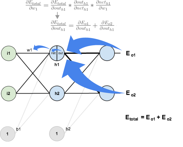
For this tutorial, we’re going to use a neural network with two inputs, two hidden neurons, two output neurons. Additionally, the hidden and output neurons will include a bias.

Here’s the basic structure:

In order to have some numbers to work with, here are the initial weights, the biases, and training inputs/outputs:

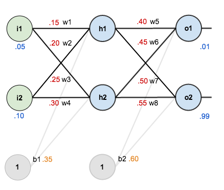
The goal of backpropagation is to optimize the weights so that the neural network can learn how to correctly map arbitrary inputs to outputs.

For the rest of this tutorial we’re going to work with a single training set: given inputs 0.05 and 0.10, we want the neural network to output 0.01 and 0.99.

The Forward Pass

To begin, lets see what the neural network currently predicts given the weights and biases above and inputs of 0.05 and 0.10. To do this we’ll feed those inputs forward though the network.

We figure out the total net input to each hidden layer neuron, squash the total net input using an activation function (here we use the logistic function), then repeat the process with the output layer neurons.

Total net input is also referred to as just net input by some sources.

Here’s how we calculate the total net input for $h_1$ :

$net_{h1} = w_1 * i_1 + w_2 * i_2 + b_1 * 1$

$net_{h1} = 0.15 * 0.05 + 0.2 * 0.1 + 0.35 * 1 = 0.3775$

We then squash it using the logistic function to get the output of $h_1$ :

$out_{h1} = \frac{1}{1+e^{-net_{h1}}} = \frac{1}{1+e^{-0.3775}} = 0.593269992$

Carrying out the same process for $h_2$ we get:

$out_{h2} = 0.596884378$

We repeat this process for the output layer neurons, using the output from the hidden layer neurons as inputs.

Here’s the output for $o_1$ :

$net_{o1} = w_5 * out_{h1} + w_6 * out_{h2} + b_2 * 1$

$net_{o1} = 0.4 * 0.593269992 + 0.45 * 0.596884378 + 0.6 * 1 = 1.105905967$

$out_{o1} = \frac{1}{1+e^{-net_{o1}}} = \frac{1}{1+e^{-1.105905967}} = 0.75136507$

And carrying out the same process for $o_2$ we get:

$out_{o2} = 0.772928465$

Calculating the Total Error

We can now calculate the error for each output neuron using the squared error function and sum them to get the total error:

$E_{total} = \sum \frac{1}{2}(target - output)^{2}$

Some sources refer to the target as the ideal and the output as the actual.

The $\frac{1}{2}$ is included so that exponent is cancelled when we differentiate later on. The result is eventually multiplied by a learning rate anyway so it doesn’t matter that we introduce a constant here [1].

For example, the target output for $o_1$ is 0.01 but the neural network output 0.75136507, therefore its error is:

$E_{o1} = \frac{1}{2}(target_{o1} - out_{o1})^{2} = \frac{1}{2}(0.01 - 0.75136507)^{2} = 0.274811083$

Repeating this process for $o_2$ (remembering that the target is 0.99) we get:

$E_{o2} = 0.023560026$

The total error for the neural network is the sum of these errors:

$E_{total} = E_{o1} + E_{o2} = 0.274811083 + 0.023560026 = 0.298371109$

The Backwards Pass

Our goal with backpropagation is to update each of the weights in the network so that they cause the actual output to be closer the target output, thereby minimizing the error for each output neuron and the network as a whole.

Output Layer

Consider $w_5$ . We want to know how much a change in $w_5$ affects the total error, aka $\frac{\partial E_{total}}{\partial w_{5}}$ .

$\frac{\partial E_{total}}{\partial w_{5}}$ is read as “the partial derivative of $E_{total}$ with respect to $w_{5}$ “. You can also say “the gradient with respect to $w_{5}$ ”.

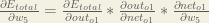
By applying the chain rule we know that:

$\frac{\partial E_{total}}{\partial w_{5}} = \frac{\partial E_{total}}{\partial out_{o1}} * \frac{\partial out_{o1}}{\partial net_{o1}} * \frac{\partial net_{o1}}{\partial w_{5}}$

Visually, here’s what we’re doing:

We need to figure out each piece in this equation.

First, how much does the total error change with respect to the output?

$E_{total} = \frac{1}{2}(target_{o1} - out_{o1})^{2} + \frac{1}{2}(target_{o2} - out_{o2})^{2}$

$\frac{\partial E_{total}}{\partial out_{o1}} = 2 * \frac{1}{2}(target_{o1} - out_{o1})^{2 - 1} * -1 + 0$

$\frac{\partial E_{total}}{\partial out_{o1}} = -(target_{o1} - out_{o1}) = -(0.01 - 0.75136507) = 0.74136507$

$-(target - out)$ is sometimes expressed as $out - target$

When we take the partial derivative of the total error with respect to $out_{o1}$ , the quantity $\frac{1}{2}(target_{o2} - out_{o2})^{2}$ becomes zero because $out_{o1}$ does not affect it which means we’re taking the derivative of a constant which is zero.

Next, how much does the output of $o_1$ change with respect to its total net input?

The partial derivative of the logistic function is the output multiplied by 1 minus the output:

$out_{o1} = \frac{1}{1+e^{-net_{o1}}}$

$\frac{\partial out_{o1}}{\partial net_{o1}} = out_{o1}(1 - out_{o1}) = 0.75136507(1 - 0.75136507) = 0.186815602$

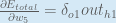
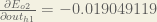
Finally, how much does the total net input of $o1$ change with respect to $w_5$ ?

$net_{o1} = w_5 * out_{h1} + w_6 * out_{h2} + b_2 * 1$

$\frac{\partial net_{o1}}{\partial w_{5}} = 1 * out_{h1} * w_5^{(1 - 1)} + 0 + 0 = out_{h1} = 0.593269992$

Putting it all together:

$\frac{\partial E_{total}}{\partial w_{5}} = \frac{\partial E_{total}}{\partial out_{o1}} * \frac{\partial out_{o1}}{\partial net_{o1}} * \frac{\partial net_{o1}}{\partial w_{5}}$

$\frac{\partial E_{total}}{\partial w_{5}} = 0.74136507 * 0.186815602 * 0.593269992 = 0.082167041$

You’ll often see this calculation combined in the form of the delta rule:

$\frac{\partial E_{total}}{\partial w_{5}} = -(target_{o1} - out_{o1}) * out_{o1}(1 - out_{o1}) * out_{h1}$

Alternatively, we have $\frac{\partial E_{total}}{\partial out_{o1}}$ and $\frac{\partial out_{o1}}{\partial net_{o1}}$ which can be written as $\frac{\partial E_{total}}{\partial net_{o1}}$ , aka $\delta_{o1}$ (the Greek letter delta) aka the node delta. We can use this to rewrite the calculation above:

$\delta_{o1} = \frac{\partial E_{total}}{\partial out_{o1}} * \frac{\partial out_{o1}}{\partial net_{o1}} = \frac{\partial E_{total}}{\partial net_{o1}}$

$\delta_{o1} = -(target_{o1} - out_{o1}) * out_{o1}(1 - out_{o1})$

Therefore:

$\frac{\partial E_{total}}{\partial w_{5}} = \delta_{o1} out_{h1}$

Some sources extract the negative sign from $\delta$ so it would be written as:

$\frac{\partial E_{total}}{\partial w_{5}} = -\delta_{o1} out_{h1}$

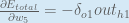
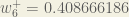
To decrease the error, we then subtract this value from the current weight (optionally multiplied by some learning rate, eta, which we’ll set to 0.5):

$w_5^{+} = w_5 - \eta * \frac{\partial E_{total}}{\partial w_{5}} = 0.4 - 0.5 * 0.082167041 = 0.35891648$

Some sources use $\alpha$ (alpha) to represent the learning rate, others use $\eta$ (eta), and others even use $\epsilon$ (epsilon).

We can repeat this process to get the new weights $w_6$ , $w_7$ , and $w_8$ :

$w_6^{+} = 0.408666186$

$w_7^{+} = 0.511301270$

$w_8^{+} = 0.561370121$

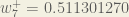
We perform the actual updates in the neural network after we have the new weights leading into the hidden layer neurons (ie, we use the original weights, not the updated weights, when we continue the backpropagation algorithm below).

Hidden Layer

Next, we’ll continue the backwards pass by calculating new values for $w_1$ , $w_2$ , $w_3$ , and $w_4$ .

Big picture, here’s what we need to figure out:

$\frac{\partial E_{total}}{\partial w_{1}} = \frac{\partial E_{total}}{\partial out_{h1}} * \frac{\partial out_{h1}}{\partial net_{h1}} * \frac{\partial net_{h1}}{\partial w_{1}}$

Visually:

We’re going to use a similar process as we did for the output layer, but slightly different to account for the fact that the output of each hidden layer neuron contributes to the output (and therefore error) of multiple output neurons. We know that $out_{h1}$ affects both $out_{o1}$ and $out_{o2}$ therefore the $\frac{\partial E_{total}}{\partial out_{h1}}$ needs to take into consideration its effect on the both output neurons:

$\frac{\partial E_{total}}{\partial out_{h1}} = \frac{\partial E_{o1}}{\partial out_{h1}} + \frac{\partial E_{o2}}{\partial out_{h1}}$

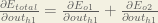
Starting with $\frac{\partial E_{o1}}{\partial out_{h1}}$ :

$\frac{\partial E_{o1}}{\partial out_{h1}} = \frac{\partial E_{o1}}{\partial net_{o1}} * \frac{\partial net_{o1}}{\partial out_{h1}}$

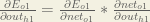
We can calculate $\frac{\partial E_{o1}}{\partial net_{o1}}$ using values we calculated earlier:

$\frac{\partial E_{o1}}{\partial net_{o1}} = \frac{\partial E_{o1}}{\partial out_{o1}} * \frac{\partial out_{o1}}{\partial net_{o1}} = 0.74136507 * 0.186815602 = 0.138498562$

And $\frac{\partial net_{o1}}{\partial out_{h1}}$ is equal to $w_5$ :

$net_{o1} = w_5 * out_{h1} + w_6 * out_{h2} + b_2 * 1$

$\frac{\partial net_{o1}}{\partial out_{h1}} = w_5 = 0.40$

Plugging them in:

$\frac{\partial E_{o1}}{\partial out_{h1}} = \frac{\partial E_{o1}}{\partial net_{o1}} * \frac{\partial net_{o1}}{\partial out_{h1}} = 0.138498562 * 0.40 = 0.055399425$

Following the same process for $\frac{\partial E_{o2}}{\partial out_{h1}}$ , we get:

$\frac{\partial E_{o2}}{\partial out_{h1}} = -0.019049119$

Therefore:

$\frac{\partial E_{total}}{\partial out_{h1}} = \frac{\partial E_{o1}}{\partial out_{h1}} + \frac{\partial E_{o2}}{\partial out_{h1}} = 0.055399425 + -0.019049119 = 0.036350306$

Now that we have $\frac{\partial E_{total}}{\partial out_{h1}}$ , we need to figure out $\frac{\partial out_{h1}}{\partial net_{h1}}$ and then $\frac{\partial net_{h1}}{\partial w}$ for each weight:

$out_{h1} = \frac{1}{1+e^{-net_{h1}}}$

$\frac{\partial out_{h1}}{\partial net_{h1}} = out_{h1}(1 - out_{h1}) = 0.59326999(1 - 0.59326999 ) = 0.241300709$

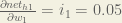
We calculate the partial derivative of the total net input to $h_1$ with respect to $w_1$ the same as we did for the output neuron:

$net_{h1} = w_1 * i_1 + w_3 * i_2 + b_1 * 1$

$\frac{\partial net_{h1}}{\partial w_1} = i_1 = 0.05$

Putting it all together:

$\frac{\partial E_{total}}{\partial w_{1}} = \frac{\partial E_{total}}{\partial out_{h1}} * \frac{\partial out_{h1}}{\partial net_{h1}} * \frac{\partial net_{h1}}{\partial w_{1}}$

$\frac{\partial E_{total}}{\partial w_{1}} = 0.036350306 * 0.241300709 * 0.05 = 0.000438568$

You might also see this written as:

$\frac{\partial E_{total}}{\partial w_{1}} = (\sum\limits_{o}{\frac{\partial E_{total}}{\partial out_{o}} * \frac{\partial out_{o}}{\partial net_{o}} * \frac{\partial net_{o}}{\partial out_{h1}}}) * \frac{\partial out_{h1}}{\partial net_{h1}} * \frac{\partial net_{h1}}{\partial w_{1}}$

$\frac{\partial E_{total}}{\partial w_{1}} = (\sum\limits_{o}{\delta_{o} * w_{ho}}) * out_{h1}(1 - out_{h1}) * i_{1}$

$\frac{\partial E_{total}}{\partial w_{1}} = \delta_{h1}i_{1}$

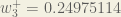
We can now update $w_1$ :

$w_1^{+} = w_1 - \eta * \frac{\partial E_{total}}{\partial w_{1}} = 0.15 - 0.5 * 0.000438568 = 0.149780716$

Repeating this for $w_2$ , $w_3$ , and $w_4$

$w_2^{+} = 0.19956143$

$w_3^{+} = 0.24975114$

$w_4^{+} = 0.29950229$

Finally, we’ve updated all of our weights! When we fed forward the 0.05 and 0.1 inputs originally, the error on the network was 0.298371109. After this first round of backpropagation, the total error is now down to 0.291027924. It might not seem like much, but after repeating this process 10,000 times, for example, the error plummets to 0.0000351085. At this point, when we feed forward 0.05 and 0.1, the two outputs neurons generate 0.015912196 (vs 0.01 target) and 0.984065734 (vs 0.99 target).

If you’ve made it this far and found any errors in any of the above or can think of any ways to make it clearer for future readers, don’t hesitate to drop me a note. Thanks!

And while I have you…

Again, if you liked this tutorial, please check out Emergent Mind, a site I’m building with an end goal of explaining AI/ML concepts in a similar style as this post. Feedback very much welcome!

1,111 thoughts on “A Step by Step Backpropagation Example”

kguzel says:

February 26, 2018 at 6:37 pm

Hi,
Thank you for this great tutorial.
if it possible, can I translate your sample to Turkish on my MEDIUM essay?
Thanks a lot.

Reply
Hans Grueber says:

February 28, 2018 at 4:41 pm

Great article, very detailed and easy to follow.

There is just something that is still unclear for me, more specifically how to calculate the new values for the biases. What bothers me is the fact that each bias is used by two neurons. For instance, b1 is used by h1 and h2.

Then, when using the partial derivative approach to come up with “correction” to the bias, should I do it with regard to h1 or with regard to h2?

Reply
David says:

March 6, 2018 at 5:24 am

Hello
I’d like to ask you when we calculate the partial derivative of E(total) with respect to out(o1), why we have to multiply it with -1.

Reply
student says:

March 6, 2018 at 7:17 am

I love you, writer. Thank you!

Reply
Jonas says:

March 6, 2018 at 1:58 pm

I really don’t understand why you calculated it this way:
E/w = E/out * out/net * net/w
instead of just calculating E/w.
E and w are still used in E/out * out/net * net/w and out/out and net/net are always 1. In addition there are more limitations (out and net have to be unequal 0).
Wouldn’t it be shorter and safer to just calculate E/w?

Reply
Michael Polkapov says:

March 10, 2018 at 11:59 pm

Thank you Very much! Really the best tutorial I have found during the search process of explanation of back propagation for dumbs. The basic has been given very Well.

Reply
Pingback: Homer Simpson Guide to Backpropagation - Sefik Ilkin Serengil
Quang Noi Truong says:

March 14, 2018 at 3:18 am

Thank for this explaination, it is helpfull for me

Reply
Satyam says:

March 15, 2018 at 12:35 pm

Can you please give an insight into momentum parameter and the math behind it with an example?

Reply
oscarjask says:

March 22, 2018 at 10:23 pm

Man this is fantastic. So good. Thank you!

Reply
Andres says:

March 27, 2018 at 10:41 am

Thank you … your explanation was very clear … it would be good if you translate it to code

Reply
student says:

March 29, 2018 at 6:43 am

This is a great tutorial, but I still can’t figure out how to apply the backward pass on multiple hidden layers. Could you please write something on this topic? Or does anyone have a good practical example for a multiple layered NN?

Reply
1. Kadmian says:
  
  April 29, 2018 at 8:25 am
  
  All you need for backpropagation with multiple layers is here.
  Try to read “next hidden layer” instead of “output layer” during the explanation of updating the hidden layer values.
  Due to the chain rule, the backpropagation process is local with respect to the layers “above” and “below” the layer you are currently processing. Said another way: what is the error of the output of a hidden layer neuron? It is the weighted sum of the node deltas of the neurons in the next layer.
  
  Reply
  1. roie says:
    
    May 27, 2018 at 12:41 pm
    
    Thank you!
    But what are the target values in this case. How should I replace the (output – target)?
    
    Reply
breezegun says:

March 31, 2018 at 8:50 am

Hi, thanks for the great guide.

This really explains when there is one instance which you have one input and one target value. What if there are multiple instances with lots of input and target pairs. Then what can one do to train the network? Train for each instance and combine the weights?

Thanks

Reply
Basit says:

April 1, 2018 at 1:56 pm

Great.it cleared all my concept.thanks

Reply
Yuki says:

April 3, 2018 at 12:00 pm

Thank you for this post ! Your explanation is very clear and easy to understand !

Reply
Joy says:

April 5, 2018 at 4:18 am

It’s so worthy to understand, Thanks :)

Reply
Pingback: Understanding Backpropagation. – A Machine Learning Blog
goksu says:

April 8, 2018 at 4:43 am

Thank you for your information about this topic. I am confused that you updated w5’s value, it became 0.3589… but later in the second part, you used w5’s value as 0.40.

Reply
1. roie says:
  
  May 27, 2018 at 12:36 pm
  
  You should use the weights before the change.
  
  Reply
Serdar says:

April 10, 2018 at 6:12 am

Thank you, now I’m able to understand what is actually going on there

Reply
Pingback: The Future of Deep Learning Research
Hotaek says:

April 13, 2018 at 4:47 am

This is really fantastic

Reply
Alejandro says:

April 14, 2018 at 2:52 pm

I was struggling to find a numeric example to practise it, thank you very much

Reply
botfactory says:

April 15, 2018 at 2:54 am

Thanks ,really help me to understand back prop

Reply
Ashutosh Chandra says:

April 15, 2018 at 2:31 pm

Awesome tutorial. I really understood ” propagating the error backwards” concept for the first time.

Reply
Bruno says:

April 18, 2018 at 3:51 am

By testing to encode the algorithm and obtaining all Wn+ correct at first update, is it possible to have a error in calculation code? My second update TotalError is wrong (0.342613).

Reply
PATRICK WONG says:

April 20, 2018 at 6:31 am

I think I’ve found an error for the partial d(out_o1)/d(net_o1). You said d(out_o1)/d(net_o1) = out_o1(1 – out_o1) but it should be d(out_o1)/d(net_o1) = net_o1 (1 – net_01). Other than that, great post!

Reply
1. PATRICK WONG says:
  
  April 21, 2018 at 8:17 pm
  
  Nevermind! Silly mistake on my part (was too tired).
  
  Reply
2. zhenxiang wang says:
  
  August 16, 2018 at 3:27 pm
  
  I think it is not correct
  Based on the chain rule, d(out_o1)/d(net_o1) should be (e^(-net_o1)/((1 + e^(-net_o1) ^ 2)
  
  Reply
  1. zhenxiang wang says:
    
    August 16, 2018 at 3:34 pm
    
    Sorry. My bad. The value is exactly same as f(x) * (1 – f(x).
    so, d(out_o1)/d(net_o1) = out_01 * (1 – out_01)
    
    Reply
Carlos says:

April 24, 2018 at 1:39 pm

I`d like to express my gratitude. I have been stuck on this Week’s. And now I think I got the basis. So I can walk without crutch and continue my course. Great explanation
Carlos valls

Reply
Pier says:

April 24, 2018 at 9:53 pm

Reblogged this on Kernel Panic.

Reply
eroidblog says:

April 25, 2018 at 10:35 pm

I finally understand! I remember bookmarking this post early this year or mid last year but I didn’t understand it. However, after brushing up on my derivatives now I do! Thank you so much for this comprehensive tutorial!

Reply
hanifanm says:

April 25, 2018 at 11:58 pm

thanks for the post :)
but what about the bias? dont we need to update it?

Reply
1. hanifanm says:
  
  April 26, 2018 at 2:57 am
  
  ive tried it, and my neural network can learn without updating the bias, thanks
  
  Reply
  1. HsintseLi says:
    
    May 8, 2018 at 6:05 am
    
    This link will show you the importance of the bias:
    https://stackoverflow.com/questions/2480650/role-of-bias-in-neural-networks
    
    Reply
  2. abeltre2050 says:
    
    May 10, 2018 at 2:17 pm
    
    It can learn without the bias, but it is not practical in larger problems. Bias needs to be updated.
    
    Reply
sanjay says:

April 30, 2018 at 6:23 am

its really helpful

Reply
Hamdy says:

May 3, 2018 at 6:28 am

Thank You…it so explanatory.

Reply
Robert Gonzalez (@3droberto) says:

May 4, 2018 at 5:46 pm

Hi Matt. Thanks you I was learn to implement it on GPU easily. https://github.com/stormcolor/gbrain
Regards ;)

Reply
HsintseLi says:

May 8, 2018 at 6:00 am

This is exactly what ‘A Step by Step Backpropagation Example’ should be! Thanks for the great post!!

Reply
Monir says:

May 11, 2018 at 2:57 am

This is indeed a very good explanation . I tried to understand andrew ng ‘s course, which is really a brilliant course. But how does back propagation derivatives works, i had some problem in understanding . This explanation makes me feel great as now i understand it fully . Thanks Mazur.

Reply
Adewole Kayode says:

May 11, 2018 at 3:14 am

This is wonderful. Thanks for the presentation. Can we then conclude that for a backpropagation algorithm to produce optimal results, the number of iterations or epoch must be large? Is there any way around this for the network to learn faster with minimum iterations? Thanks.

Reply
Hanbit, Lee says:

May 11, 2018 at 6:53 am

I’m korean. Your explanation is best of best!
Thank you for ginving this story.

Reply
koushik says:

May 11, 2018 at 11:38 am

you are not updated the bias ,please ensure me that it is necessary or not.

Reply
Juel Khan says:

May 12, 2018 at 1:21 am

Your explanation is awesome. Thanks a lot.

Reply
Jerome Paddick says:

May 14, 2018 at 12:24 pm

I was really struggling with this, thanks for breaking it down and explaining it so well !

Reply
Nikhil Varma says:

May 17, 2018 at 8:05 am

Hey,
A really great explanation, thanks for sharing the knowledge.

Reply
Dave C says:

May 24, 2018 at 10:34 am

so glad i stumbled across this site! youre my new fav blog as im a mechanical engineer shifting more towards data science/deep learning for autonomous vehicles and i enjoy playing NLHE – one stop shop for all my interests! got a lot of old posts to sift through – great work and documentation! very good simple explanations and a nice clean layout – keep up the good work!

Reply
Ashutosh kushwaha says:

May 29, 2018 at 12:58 am

For multi-class classification with neural networks having regularisation parameter, we have a different kind of cost function involving each and every weight and term including regularisation parameter multiplied with weights, does this regularisation parameter will affect the backpropagation algorithm????

Reply
Neda says:

May 31, 2018 at 10:01 am

I have written the corresponding code for a 4-7-2 network. the training mean squared error decreases well but the problem is that when I apply the updated weights and biases to the network at each iteration in order to check the validation error (the validation data set is applied randomly), the validation error increases badly. that is why the test fails. I do not have any idea what is the reason behind this.
I was wondering if somebody gives me some advice to deal with such issue.
Thanks

Reply
Vendidad says:

June 3, 2018 at 1:00 am

Very detailed & thorough explanation … much appreciated! Python code to implement this example. I am not a developer, so am sure there are more efficient/elegant ways of coding this.
https://github.com/vendidad/DS-repo/blob/master/Backpropagation%20-%20Consolidated%20Script.ipynb

Reply
Dominic Pritham says:

June 8, 2018 at 11:39 am

Hi Matt:

Thank you very much for this awesome explanation.
A major component Back propagation is finding out how a weight affects total error, correct?
With that being said, from the breakdown of dEtotal/dw5, the only factor that involves w5 is dnetout/dw5. But this simply breaks down to hout1. I am failing to see how tweaking of w5 is done here, aside from w5+ = w5 – alpha(dEotal/dw5).
My question is also more geared towards what happens when the weight we compute increases the total error.

Reply
Saliya says:

June 11, 2018 at 4:00 pm

This is great! Thank you for the step by step explanation

Reply
Hasan says:

June 13, 2018 at 3:36 am

Fantastic write up. Many thanks.

Reply
Pingback: 機器學習-積累與發現繼續 - 程序員的後花園
Joe says:

June 20, 2018 at 6:42 am

Do you really update the link weights by just subtracting the update from the last weight? I am asking because I have just repreduced the example and after 10,000 iteration some weights go into the -3 and 2 area. If I look at the equations it seems to confirm that there is nothing that prevents this.

I was under the impression that both link and node weights need to be in the 0,1 or -1,1 interval. Maybe this assumption is wrong?

Reply