A Step by Step Backpropagation Example

March 17, 2015February 23, 2024Mazur

Background

Backpropagation is a common method for training a neural network. There is no shortage of papers online that attempt to explain how backpropagation works, but few that include an example with actual numbers. This post is my attempt to explain how it works with a concrete example that folks can compare their own calculations to in order to ensure they understand backpropagation correctly.

Backpropagation in Python

You can play around with a Python script that I wrote that implements the backpropagation algorithm in this Github repo.

Continue learning with Emergent Mind

If you find this tutorial useful and want to continue learning about AI/ML, I encourage you to check out Emergent Mind, a new website I’m working on that uses GPT-4 to surface and explain cutting-edge AI/ML papers:

In time, I hope to use AI to explain complex AI/ML topics on Emergent Mind in a style similar to what you’ll find in the tutorial below.

Now, on with the backpropagation tutorial…

Overview

For this tutorial, we’re going to use a neural network with two inputs, two hidden neurons, two output neurons. Additionally, the hidden and output neurons will include a bias.

Here’s the basic structure:

In order to have some numbers to work with, here are the initial weights, the biases, and training inputs/outputs:

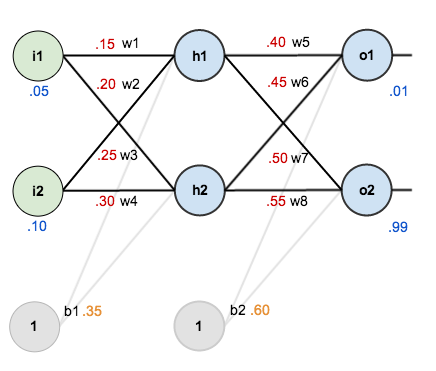
The goal of backpropagation is to optimize the weights so that the neural network can learn how to correctly map arbitrary inputs to outputs.

For the rest of this tutorial we’re going to work with a single training set: given inputs 0.05 and 0.10, we want the neural network to output 0.01 and 0.99.

The Forward Pass

To begin, lets see what the neural network currently predicts given the weights and biases above and inputs of 0.05 and 0.10. To do this we’ll feed those inputs forward though the network.

We figure out the total net input to each hidden layer neuron, squash the total net input using an activation function (here we use the logistic function), then repeat the process with the output layer neurons.

Total net input is also referred to as just net input by some sources.

Here’s how we calculate the total net input for $h_1$ :

$net_{h1} = w_1 * i_1 + w_2 * i_2 + b_1 * 1$

$net_{h1} = 0.15 * 0.05 + 0.2 * 0.1 + 0.35 * 1 = 0.3775$

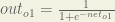
We then squash it using the logistic function to get the output of $h_1$ :

$out_{h1} = \frac{1}{1+e^{-net_{h1}}} = \frac{1}{1+e^{-0.3775}} = 0.593269992$

Carrying out the same process for $h_2$ we get:

$out_{h2} = 0.596884378$

We repeat this process for the output layer neurons, using the output from the hidden layer neurons as inputs.

Here’s the output for $o_1$ :

$net_{o1} = w_5 * out_{h1} + w_6 * out_{h2} + b_2 * 1$

$net_{o1} = 0.4 * 0.593269992 + 0.45 * 0.596884378 + 0.6 * 1 = 1.105905967$

$out_{o1} = \frac{1}{1+e^{-net_{o1}}} = \frac{1}{1+e^{-1.105905967}} = 0.75136507$

And carrying out the same process for $o_2$ we get:

$out_{o2} = 0.772928465$

Calculating the Total Error

We can now calculate the error for each output neuron using the squared error function and sum them to get the total error:

$E_{total} = \sum \frac{1}{2}(target - output)^{2}$

Some sources refer to the target as the ideal and the output as the actual.

The $\frac{1}{2}$ is included so that exponent is cancelled when we differentiate later on. The result is eventually multiplied by a learning rate anyway so it doesn’t matter that we introduce a constant here [1].

For example, the target output for $o_1$ is 0.01 but the neural network output 0.75136507, therefore its error is:

$E_{o1} = \frac{1}{2}(target_{o1} - out_{o1})^{2} = \frac{1}{2}(0.01 - 0.75136507)^{2} = 0.274811083$

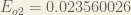
Repeating this process for $o_2$ (remembering that the target is 0.99) we get:

$E_{o2} = 0.023560026$

The total error for the neural network is the sum of these errors:

$E_{total} = E_{o1} + E_{o2} = 0.274811083 + 0.023560026 = 0.298371109$

The Backwards Pass

Our goal with backpropagation is to update each of the weights in the network so that they cause the actual output to be closer the target output, thereby minimizing the error for each output neuron and the network as a whole.

Output Layer

Consider $w_5$ . We want to know how much a change in $w_5$ affects the total error, aka $\frac{\partial E_{total}}{\partial w_{5}}$ .

$\frac{\partial E_{total}}{\partial w_{5}}$ is read as “the partial derivative of $E_{total}$ with respect to $w_{5}$ “. You can also say “the gradient with respect to $w_{5}$ ”.

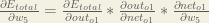
By applying the chain rule we know that:

$\frac{\partial E_{total}}{\partial w_{5}} = \frac{\partial E_{total}}{\partial out_{o1}} * \frac{\partial out_{o1}}{\partial net_{o1}} * \frac{\partial net_{o1}}{\partial w_{5}}$

Visually, here’s what we’re doing:

We need to figure out each piece in this equation.

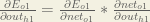
First, how much does the total error change with respect to the output?

$E_{total} = \frac{1}{2}(target_{o1} - out_{o1})^{2} + \frac{1}{2}(target_{o2} - out_{o2})^{2}$

$\frac{\partial E_{total}}{\partial out_{o1}} = 2 * \frac{1}{2}(target_{o1} - out_{o1})^{2 - 1} * -1 + 0$

$\frac{\partial E_{total}}{\partial out_{o1}} = -(target_{o1} - out_{o1}) = -(0.01 - 0.75136507) = 0.74136507$

$-(target - out)$ is sometimes expressed as $out - target$

When we take the partial derivative of the total error with respect to $out_{o1}$ , the quantity $\frac{1}{2}(target_{o2} - out_{o2})^{2}$ becomes zero because $out_{o1}$ does not affect it which means we’re taking the derivative of a constant which is zero.

Next, how much does the output of $o_1$ change with respect to its total net input?

The partial derivative of the logistic function is the output multiplied by 1 minus the output:

$out_{o1} = \frac{1}{1+e^{-net_{o1}}}$

$\frac{\partial out_{o1}}{\partial net_{o1}} = out_{o1}(1 - out_{o1}) = 0.75136507(1 - 0.75136507) = 0.186815602$

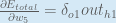
Finally, how much does the total net input of $o1$ change with respect to $w_5$ ?

$net_{o1} = w_5 * out_{h1} + w_6 * out_{h2} + b_2 * 1$

$\frac{\partial net_{o1}}{\partial w_{5}} = 1 * out_{h1} * w_5^{(1 - 1)} + 0 + 0 = out_{h1} = 0.593269992$

Putting it all together:

$\frac{\partial E_{total}}{\partial w_{5}} = \frac{\partial E_{total}}{\partial out_{o1}} * \frac{\partial out_{o1}}{\partial net_{o1}} * \frac{\partial net_{o1}}{\partial w_{5}}$

$\frac{\partial E_{total}}{\partial w_{5}} = 0.74136507 * 0.186815602 * 0.593269992 = 0.082167041$

You’ll often see this calculation combined in the form of the delta rule:

$\frac{\partial E_{total}}{\partial w_{5}} = -(target_{o1} - out_{o1}) * out_{o1}(1 - out_{o1}) * out_{h1}$

Alternatively, we have $\frac{\partial E_{total}}{\partial out_{o1}}$ and $\frac{\partial out_{o1}}{\partial net_{o1}}$ which can be written as $\frac{\partial E_{total}}{\partial net_{o1}}$ , aka $\delta_{o1}$ (the Greek letter delta) aka the node delta. We can use this to rewrite the calculation above:

$\delta_{o1} = \frac{\partial E_{total}}{\partial out_{o1}} * \frac{\partial out_{o1}}{\partial net_{o1}} = \frac{\partial E_{total}}{\partial net_{o1}}$

$\delta_{o1} = -(target_{o1} - out_{o1}) * out_{o1}(1 - out_{o1})$

Therefore:

$\frac{\partial E_{total}}{\partial w_{5}} = \delta_{o1} out_{h1}$

Some sources extract the negative sign from $\delta$ so it would be written as:

$\frac{\partial E_{total}}{\partial w_{5}} = -\delta_{o1} out_{h1}$

To decrease the error, we then subtract this value from the current weight (optionally multiplied by some learning rate, eta, which we’ll set to 0.5):

$w_5^{+} = w_5 - \eta * \frac{\partial E_{total}}{\partial w_{5}} = 0.4 - 0.5 * 0.082167041 = 0.35891648$

Some sources use $\alpha$ (alpha) to represent the learning rate, others use $\eta$ (eta), and others even use $\epsilon$ (epsilon).

We can repeat this process to get the new weights $w_6$ , $w_7$ , and $w_8$ :

$w_6^{+} = 0.408666186$

$w_7^{+} = 0.511301270$

$w_8^{+} = 0.561370121$

We perform the actual updates in the neural network after we have the new weights leading into the hidden layer neurons (ie, we use the original weights, not the updated weights, when we continue the backpropagation algorithm below).

Hidden Layer

Next, we’ll continue the backwards pass by calculating new values for $w_1$ , $w_2$ , $w_3$ , and $w_4$ .

Big picture, here’s what we need to figure out:

$\frac{\partial E_{total}}{\partial w_{1}} = \frac{\partial E_{total}}{\partial out_{h1}} * \frac{\partial out_{h1}}{\partial net_{h1}} * \frac{\partial net_{h1}}{\partial w_{1}}$

Visually:

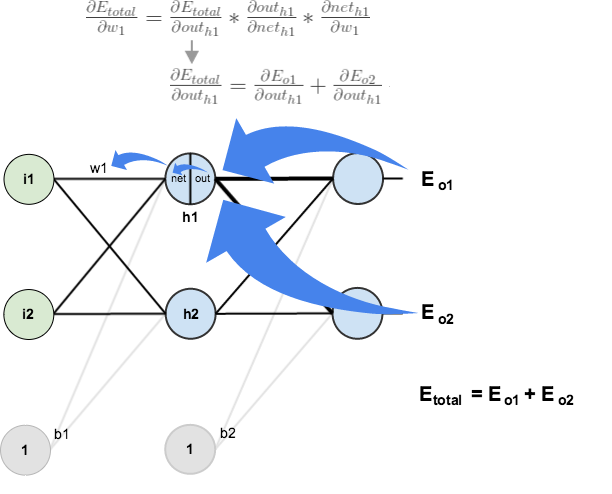
We’re going to use a similar process as we did for the output layer, but slightly different to account for the fact that the output of each hidden layer neuron contributes to the output (and therefore error) of multiple output neurons. We know that $out_{h1}$ affects both $out_{o1}$ and $out_{o2}$ therefore the $\frac{\partial E_{total}}{\partial out_{h1}}$ needs to take into consideration its effect on the both output neurons:

$\frac{\partial E_{total}}{\partial out_{h1}} = \frac{\partial E_{o1}}{\partial out_{h1}} + \frac{\partial E_{o2}}{\partial out_{h1}}$

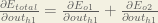
Starting with $\frac{\partial E_{o1}}{\partial out_{h1}}$ :

$\frac{\partial E_{o1}}{\partial out_{h1}} = \frac{\partial E_{o1}}{\partial net_{o1}} * \frac{\partial net_{o1}}{\partial out_{h1}}$

We can calculate $\frac{\partial E_{o1}}{\partial net_{o1}}$ using values we calculated earlier:

$\frac{\partial E_{o1}}{\partial net_{o1}} = \frac{\partial E_{o1}}{\partial out_{o1}} * \frac{\partial out_{o1}}{\partial net_{o1}} = 0.74136507 * 0.186815602 = 0.138498562$

And $\frac{\partial net_{o1}}{\partial out_{h1}}$ is equal to $w_5$ :

$net_{o1} = w_5 * out_{h1} + w_6 * out_{h2} + b_2 * 1$

$\frac{\partial net_{o1}}{\partial out_{h1}} = w_5 = 0.40$

Plugging them in:

$\frac{\partial E_{o1}}{\partial out_{h1}} = \frac{\partial E_{o1}}{\partial net_{o1}} * \frac{\partial net_{o1}}{\partial out_{h1}} = 0.138498562 * 0.40 = 0.055399425$

Following the same process for $\frac{\partial E_{o2}}{\partial out_{h1}}$ , we get:

$\frac{\partial E_{o2}}{\partial out_{h1}} = -0.019049119$

Therefore:

$\frac{\partial E_{total}}{\partial out_{h1}} = \frac{\partial E_{o1}}{\partial out_{h1}} + \frac{\partial E_{o2}}{\partial out_{h1}} = 0.055399425 + -0.019049119 = 0.036350306$

Now that we have $\frac{\partial E_{total}}{\partial out_{h1}}$ , we need to figure out $\frac{\partial out_{h1}}{\partial net_{h1}}$ and then $\frac{\partial net_{h1}}{\partial w}$ for each weight:

$out_{h1} = \frac{1}{1+e^{-net_{h1}}}$

$\frac{\partial out_{h1}}{\partial net_{h1}} = out_{h1}(1 - out_{h1}) = 0.59326999(1 - 0.59326999 ) = 0.241300709$

We calculate the partial derivative of the total net input to $h_1$ with respect to $w_1$ the same as we did for the output neuron:

$net_{h1} = w_1 * i_1 + w_3 * i_2 + b_1 * 1$

$\frac{\partial net_{h1}}{\partial w_1} = i_1 = 0.05$

Putting it all together:

$\frac{\partial E_{total}}{\partial w_{1}} = \frac{\partial E_{total}}{\partial out_{h1}} * \frac{\partial out_{h1}}{\partial net_{h1}} * \frac{\partial net_{h1}}{\partial w_{1}}$

$\frac{\partial E_{total}}{\partial w_{1}} = 0.036350306 * 0.241300709 * 0.05 = 0.000438568$

You might also see this written as:

$\frac{\partial E_{total}}{\partial w_{1}} = (\sum\limits_{o}{\frac{\partial E_{total}}{\partial out_{o}} * \frac{\partial out_{o}}{\partial net_{o}} * \frac{\partial net_{o}}{\partial out_{h1}}}) * \frac{\partial out_{h1}}{\partial net_{h1}} * \frac{\partial net_{h1}}{\partial w_{1}}$

$\frac{\partial E_{total}}{\partial w_{1}} = (\sum\limits_{o}{\delta_{o} * w_{ho}}) * out_{h1}(1 - out_{h1}) * i_{1}$

$\frac{\partial E_{total}}{\partial w_{1}} = \delta_{h1}i_{1}$

We can now update $w_1$ :

$w_1^{+} = w_1 - \eta * \frac{\partial E_{total}}{\partial w_{1}} = 0.15 - 0.5 * 0.000438568 = 0.149780716$

Repeating this for $w_2$ , $w_3$ , and $w_4$

$w_2^{+} = 0.19956143$

$w_3^{+} = 0.24975114$

$w_4^{+} = 0.29950229$

Finally, we’ve updated all of our weights! When we fed forward the 0.05 and 0.1 inputs originally, the error on the network was 0.298371109. After this first round of backpropagation, the total error is now down to 0.291027924. It might not seem like much, but after repeating this process 10,000 times, for example, the error plummets to 0.0000351085. At this point, when we feed forward 0.05 and 0.1, the two outputs neurons generate 0.015912196 (vs 0.01 target) and 0.984065734 (vs 0.99 target).

If you’ve made it this far and found any errors in any of the above or can think of any ways to make it clearer for future readers, don’t hesitate to drop me a note. Thanks!

And while I have you…

Again, if you liked this tutorial, please check out Emergent Mind, a site I’m building with an end goal of explaining AI/ML concepts in a similar style as this post. Feedback very much welcome!

1,090 thoughts on “A Step by Step Backpropagation Example”

chantiq1000x says:

June 21, 2018 at 9:44 am

can you tell me why h1 = w1*x1 + w2*x2 +b ? why not h1 = w1 * x1 + w3* x3 + b

Reply
1. Joseph says:
  
  August 1, 2018 at 9:28 pm
  
  The labeling is slightly ambiguous because the weights were not put right on top of the links/edges. w2 is not going from i1 to h2, it is going from i2 to h1. That is, the weights are labeled to the left of their respective links/edges, not to the right. This is a little bit more obvious in the first graph.
  
  Reply
George Skrimpas says:

June 21, 2018 at 12:23 pm

I think the correct formula for H1 is:
netH1 = w1*i1 + w3*i2 + b1*1
i use w3 instead of w2, since I2 is linked to H1 via w3.
Will you plz confirm?

Reply
1. Jeremiah says:
  
  February 8, 2019 at 10:01 am
  
  No the way the math is done by the author is the correct one.. Use the equations in order to understand the graph
  
  Reply
deepak says:

June 27, 2018 at 11:31 am

many errors dude mainly the computation of d(h1)/d(o2))=-(0.01 – 0.772928465)*(0.772928465*(1-0.772928465))*0.45

Reply
Suman says:

June 30, 2018 at 4:06 pm

It really helped me to understand how back propagation works. Keep up the good work.

Reply
mcavidya says:

July 3, 2018 at 9:11 pm

Thanks Mazur for this numerical example. Such an example provides the best way to learn the working of an algorithm. It helped me a lot. Many thanks.
Going through the example, I was wondering whether the biases b1, b2 are being treated as constants. Is it not necessary to adjust their values also?

Reply
1. Mayank Gupta says:
  
  August 6, 2018 at 5:10 am
  
  Yes. In this article, biases were treated as constants to keep things simple. If you understood the math explained in this article, you can easily update the biases as well. In reality, biases are also updated.
  
  Reply
  1. enginbozaba says:
    
    September 11, 2018 at 1:24 pm
    
    Are we updating the bias values by setting up the dE / db1 and dE / db2 chains?
    
    Reply
Pony says:

July 3, 2018 at 10:16 pm

This is great! Thank you for the step by step explanation

Reply
Jerome lemoine says:

July 6, 2018 at 3:04 pm

Hi matt
Great document, very pedagogic !
Maybe a little mistake in the calculation of the net_h1 and net_h2:
net_h1= w1×i1 + w3×i3 + b1
(Analog mistake for net_h2)
The mistake is communicated to the numerical application also

Reply
lamductan says:

July 25, 2018 at 4:56 am

This explaination and visualization is very well understanding. It helps me so much because it takes me a lot of time to know how really backpropagation does. Thank you very much.

Reply
Pingback: A Step by Step Backpropagation Example – Deep Learning
jeffminich says:

July 31, 2018 at 5:21 pm

Outstanding explainer for back propagation. Thanks, Matt!

Reply
Mayank Gupta says:

August 6, 2018 at 5:07 am

I was a bit frustrated with this backpropagation topic and was struggling to have a clear mental picture of backpropagation.

Your article radically improved my understanding. Your article was so clear that I was actually able to write my own code to implement backpropagation. Thank you very much.

If you ever plan to expand on this article, I request you to add some details about how weights are updated for all the samples (your article explained the case for one sample.)

Thanks again for this wonderful article!

Reply
arnulfo says:

August 6, 2018 at 11:07 pm

Reblogged this on conlatio.

Reply
Amin says:

August 7, 2018 at 9:51 am

Goog job! But this is 3-layer network only. If it is 4-layer then how we calculate the dEtotal/dout(h1)?

dEh2/dout(h1) will not be know. Because we don’t have the value for dEh2 (the error for hidden layer 2). I need an explanation here. Thanks!

Reply
1. Zhijie Chen says:
  
  August 15, 2018 at 11:12 am
  
  You use the value that comes from the previous layer. For instance dE/dout i1 = dE/dnet h1 * dnet h1/ dout i1 = dE/dout h1 * dout h1 / dnet h1 * dnet h1/dout i1, in which dE/dout h1 and dout h1 / dnet h1 have been calculated by the previous layer.
  
  Reply
  1. Knut Leiß says:
    
    November 14, 2018 at 4:36 am
    
    I got the same problem and I don’t understand the answer.
    Why is dE/dout i1 =dE/dnet h1 * dnet h1/dout i1?
    This ignores the contribution of out i1 to the error through h2!?
    So, I assume the term dE/dnet h2 * dnet h2/dout i1 needs to be added!? But then, why is it OK to just use the sum, mathematically?
    
    Reply
Frank says:

August 15, 2018 at 3:27 pm

Question: do all neurons in a layer use the same bias weight or is there a individual weight per neuron? I.e. In the example it looks like that b1 is used for both hidden neurons and b2 for both output neurons.

Btw: nice and easy to follow example!

Reply
1. Aaron says:
  
  October 23, 2018 at 1:20 am
  
  In reality each bias would be adjusted too, but in the example seems like they are only focusing on weights, and specifically the hidden layers.
  
  Reply
2. Hazem says:
  
  December 18, 2018 at 7:12 am
  
  Yes, all neurons in a layer use the same bias weight
  
  Reply
Pingback: Implementing a flexible neural network with backpropagation from scratch
anil says:

August 21, 2018 at 12:03 am

i think this is best explain backpropagation with detail kudos!

Reply
Pingback: Important Links | Tejalal Choudhary
Garrett says:

August 24, 2018 at 11:07 pm

This was a fantastic write up. I am using it to study the algorithm while currently in an AI course at uni. I was wondering if you could add to this and describe momentum in the same way. Thank you

Reply
Rafay says:

August 27, 2018 at 1:09 pm

Thanks a lot Matt for making this. Your blog and the Stanford’s CS231n lectures are the best resources on this.

Reply
Pingback: Deep learning for product managers – part 1 – Kai's notebook
Alan Wake says:

August 31, 2018 at 7:52 am

Thank you very much! I’ve been looking exactly for this

Reply
Pingback: 【每日AI收集】BP神经网络 - 每日AI
Sneha says:

September 9, 2018 at 5:07 am

This page is very helpful to solve the problems.
Amazing page !!
Thank you !!

Reply
Kevin says:

September 15, 2018 at 1:22 am

Thanks for the great example. One question though:
During the backpropagation, you find the new values for w5-w8 and continue backpropagating the previous hidden layer. There you need the value of dnet_o1/dout_h1, which equals w5. Do we use the original value of w5, 0.4, as it is done here or its updated value, 0.35891648 ?

Reply
1. todd_wang says:
  
  November 28, 2018 at 12:44 pm
  
  Backpropagation is based on previous forwordpropagation, so w5 should be same as original w5 rather than updated one.
  
  Reply
Artem says:

September 15, 2018 at 12:20 pm

Thank you for explanation. I didn’t get one thing. Why we multyply by -1 derivative of totel error? is this because target is constant and out1 is function?

Reply
1. thegopieffect says:
  
  December 23, 2018 at 10:01 am
  
  Hey did you found why derivative for out1 is multiplied by -1 ??
  
  Reply
Abin Singh says:

September 21, 2018 at 4:08 am

You said in the beginning that we are going to work with only a single training set (1 row with 2 features ). Then how we are getting two outputs. It should be one right.

Can you please clarify?

Reply
1. Braydon Burkhardt says:
  
  November 27, 2018 at 1:40 pm
  
  Training sets can have as many inputs and outputs as you want. What the “1 row with 2 features” means is that there is only 1 training set in the entire list. For example if you input a (0,1), it will output a (0.5,0.5). For 2 ‘rows’ or training sets, you can have (0,1)->(0.5,0.5) OR if it is for example a (1,1)->(0.6,0.2). The row means a new ‘if’ statement. I am not sure what you mean by ‘feature’ if you’re talking about the amount of hidden neurons, the average between input/output neurons, or the amount of biases.
  
  Reply
Jimmy Johnson says:

September 25, 2018 at 1:00 am

Very nice explanation.
Thanks for taking the time to do this.

Reply
swapna says:

September 27, 2018 at 9:36 am

its really very helpful..thanks for such a wonderful doc

Reply
ynot werk says:

September 29, 2018 at 3:14 pm

Carrying out the same process for h_2 we get:

out_{h2} = 0.596884378

I got 0.666522 for h2 because i did: activation_function(0.25 * 0.05 + 0.3 * 0.1 + 0.65 * 1)

Reply
R S SARATHI KANNAN says:

October 5, 2018 at 11:52 pm

Hi,
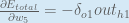
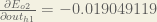
It is a good work. I am struck at here, Following the same process for \frac{\partial E_{o2}}{\partial out_{h1}}, we get:

\frac{\partial E_{o2}}{\partial out_{h1}} = -0.019049119 (partial derivative of H1out from E2)… how to calculate out_H1 from E2

Reply
Martin Ennemoser says:

October 13, 2018 at 4:10 am

Thanks for this awesome explanation.

Reply
Kartikey arora says:

October 18, 2018 at 10:54 am

This article was really very helpful for me as i was very confused and stuck with tha backprop calculations and u just explained it with an example in a very nice way thanks a lot

Reply
Pingback: A simple natural language category classifier with Keras – GrownSoftware
Ravi says:

October 21, 2018 at 3:51 am

Final wieghts after 10,000 iterations are
0.378509988350132
0.657019976700263
0.477300705684786
0.754601411369569
-3.892977198865724
-3.868416687703616
2.861810948620059
2.925688966771616

Reply
1. Ana says:
  
  October 30, 2018 at 2:23 pm
  
  I’ve got the same, is that right? aren’t weights supposed to be between 1-10?
  
  Reply
  1. Braydon Burkhardt says:
    
    January 10, 2019 at 10:15 pm
    
    weights can be any number, but the larger the absolute of it is, the longer it will to calculate.
    
    Reply
Pingback: Neuronal networking in VBA+Excel
Aaron says:

October 22, 2018 at 11:01 pm

This is an awesome post, I was confused about how the error propagates through the hidden layer. Working through each step made the equations seem intuitive. Someone should really make an animation for this.

Reply
Pingback: [D] Is there a book or resource about machine learning that teaches different algorithms with step by step calculations for simple examples? Like how a mathematics or physics book would. | Premium Blog! | Development code, Android, Ios anh Tranning IT
Raja says:

October 24, 2018 at 7:16 pm

Hi Experts, I tried this approach, for some reason my weights and error keeps increasing, doesn’t seem to reduce for certain inputs, any idea whats happening ?

Reply
eduhelp2016 says:

October 27, 2018 at 5:47 am

Lovely!!!!!!!!!!!

Reply
T.smart says:

October 29, 2018 at 3:08 am

it is my answer,
0 0.291027774
1 0.283547133
2 0.275943289
3 0.268232761
4 0.260434393
5 0.252569176
6 0.244659999
7 0.236731316
8 0.228808741
9 0.220918592
10 0.213087389
11 0.205341328
12 0.197705769
13 0.190204742
14 0.182860503
15 0.175693166
16 0.168720403
17 0.16195725
18 0.155415989
19 0.149106135
20 0.14303449
21 0.137205276
22 0.131620316
23 0.126279262
24 0.121179847
25 0.116318143
26 0.111688831
27 0.107285459
28 0.103100677
29 0.099126464
30 0.095354325
31 0.091775464
32 0.088380932
33 0.085161757
34 0.082109043
I am not sure that it is right.

Reply
PARAMESHA K says:

October 31, 2018 at 9:05 pm

Whether the BP should run far all the training samples or individual samples?

Reply
Pingback: Understanding Evolved Policy Gradients – AI+ NEWS
purnenduprabhat says:

November 11, 2018 at 3:38 am

Excellent explanation! Cleared my doubt.

Reply
Sebastian says:

November 11, 2018 at 9:45 am

Great explanation. Thanks. Many authors who write books consider themselves as being smart just because they provide some complicated formulas from wikipedia with 10,000 different index symbols. But I do not think they are smart at all. They do not know their audience. This simple example is better than all books that I have which try to explain back propagation with fomrulas… I did not realize it is that simple. It is just taking derivative over and over again. Thank you very much!

Reply
Santiago Fernando Gomez says:

November 19, 2018 at 5:22 pm

This is amazing, the best explanation I have found over the internet. Great job!

Reply
Dariusz Tomaszewski says:

November 23, 2018 at 5:13 pm

Great explanation Matt. The best I have seen so far.

Reply
Mojtaba Sabbagh says:

November 30, 2018 at 5:54 am

Thanks, Very clear and useful.

Reply
Hai Ha says:

December 3, 2018 at 11:08 pm

Thank you very much but I have a question.
At the beginning w1 = 0.15, w2 = 0.2, b1 = 0.35 => How to initialize these weight, bias values.
=> How to nit matrix of Height, Bias ?

Reply
Peter says:

December 4, 2018 at 12:15 am

Great explanation. I had no problem following your description, but I am missing a critical piece. In reality, we always have more than 1 row of inputs and outputs for training data (we could have hundreds of thousands of rows). How does this then affect the computations of the derivatives? I’m sure all training rows play into the total error, but I am missing what is probably a simple connection on calculating new weights in light of all the data. Can you explain how you would get the updated weights if you had two rows of training data? Do you process it one row at a time and then average the new computed weights together to determine the updated values? Is there a fast way to do this?

Reply
Agi Maulana says:

December 4, 2018 at 9:03 am

Very good explanation. Thank you, it’s so useful for me. Now, the problem is on me, I must improve my math skill.

Reply