A Step by Step Backpropagation Example

Background

Backpropagation is a common method for training a neural network. There is no shortage of papers online that attempt to explain how backpropagation works, but few that include an example with actual numbers. This post is my attempt to explain how it works with a concrete example that folks can compare their own calculations to in order to ensure they understand backpropagation correctly.

Backpropagation in Python

You can play around with a Python script that I wrote that implements the backpropagation algorithm in this Github repo.

Backpropagation Visualization

For an interactive visualization showing a neural network as it learns, check out my Neural Network visualization.

Additional Resources

If you find this tutorial useful and want to continue learning about neural networks, machine learning, and deep learning, I highly recommend checking out Adrian Rosebrock’s new book, Deep Learning for Computer Vision with Python. I really enjoyed the book and will have a full review up soon.

Overview

For this tutorial, we’re going to use a neural network with two inputs, two hidden neurons, two output neurons. Additionally, the hidden and output neurons will include a bias.

Here’s the basic structure:

neural_network (7)

In order to have some numbers to work with, here are the initial weights, the biases, and training inputs/outputs:

neural_network (9)

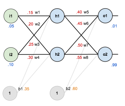
The goal of backpropagation is to optimize the weights so that the neural network can learn how to correctly map arbitrary inputs to outputs.

For the rest of this tutorial we’re going to work with a single training set: given inputs 0.05 and 0.10, we want the neural network to output 0.01 and 0.99.

The Forward Pass

To begin, lets see what the neural network currently predicts given the weights and biases above and inputs of 0.05 and 0.10. To do this we’ll feed those inputs forward though the network.

We figure out the total net input to each hidden layer neuron, squash the total net input using an activation function (here we use the logistic function), then repeat the process with the output layer neurons.

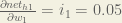
Total net input is also referred to as just net input by some sources.

Here’s how we calculate the total net input for $h_1$ :

$net_{h1} = w_1 * i_1 + w_2 * i_2 + b_1 * 1$

$net_{h1} = 0.15 * 0.05 + 0.2 * 0.1 + 0.35 * 1 = 0.3775$

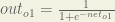
We then squash it using the logistic function to get the output of $h_1$ :

$out_{h1} = \frac{1}{1+e^{-net_{h1}}} = \frac{1}{1+e^{-0.3775}} = 0.593269992$

Carrying out the same process for $h_2$ we get:

$out_{h2} = 0.596884378$

We repeat this process for the output layer neurons, using the output from the hidden layer neurons as inputs.

Here’s the output for $o_1$ :

$net_{o1} = w_5 * out_{h1} + w_6 * out_{h2} + b_2 * 1$

$net_{o1} = 0.4 * 0.593269992 + 0.45 * 0.596884378 + 0.6 * 1 = 1.105905967$

$out_{o1} = \frac{1}{1+e^{-net_{o1}}} = \frac{1}{1+e^{-1.105905967}} = 0.75136507$

And carrying out the same process for $o_2$ we get:

$out_{o2} = 0.772928465$

Calculating the Total Error

We can now calculate the error for each output neuron using the squared error function and sum them to get the total error:

$E_{total} = \sum \frac{1}{2}(target - output)^{2}$

Some sources refer to the target as the ideal and the output as the actual.

The $\frac{1}{2}$ is included so that exponent is cancelled when we differentiate later on. The result is eventually multiplied by a learning rate anyway so it doesn’t matter that we introduce a constant here [1].

For example, the target output for $o_1$ is 0.01 but the neural network output 0.75136507, therefore its error is:

$E_{o1} = \frac{1}{2}(target_{o1} - out_{o1})^{2} = \frac{1}{2}(0.01 - 0.75136507)^{2} = 0.274811083$

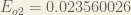
Repeating this process for $o_2$ (remembering that the target is 0.99) we get:

$E_{o2} = 0.023560026$

The total error for the neural network is the sum of these errors:

$E_{total} = E_{o1} + E_{o2} = 0.274811083 + 0.023560026 = 0.298371109$

The Backwards Pass

Our goal with backpropagation is to update each of the weights in the network so that they cause the actual output to be closer the target output, thereby minimizing the error for each output neuron and the network as a whole.

Output Layer

Consider $w_5$ . We want to know how much a change in $w_5$ affects the total error, aka $\frac{\partial E_{total}}{\partial w_{5}}$ .

$\frac{\partial E_{total}}{\partial w_{5}}$ is read as “the partial derivative of $E_{total}$ with respect to $w_{5}$ “. You can also say “the gradient with respect to $w_{5}$ “.

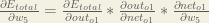
By applying the chain rule we know that:

$\frac{\partial E_{total}}{\partial w_{5}} = \frac{\partial E_{total}}{\partial out_{o1}} * \frac{\partial out_{o1}}{\partial net_{o1}} * \frac{\partial net_{o1}}{\partial w_{5}}$

Visually, here’s what we’re doing:

output_1_backprop (4)

We need to figure out each piece in this equation.

First, how much does the total error change with respect to the output?

$E_{total} = \frac{1}{2}(target_{o1} - out_{o1})^{2} + \frac{1}{2}(target_{o2} - out_{o2})^{2}$

$\frac{\partial E_{total}}{\partial out_{o1}} = 2 * \frac{1}{2}(target_{o1} - out_{o1})^{2 - 1} * -1 + 0$

$\frac{\partial E_{total}}{\partial out_{o1}} = -(target_{o1} - out_{o1}) = -(0.01 - 0.75136507) = 0.74136507$

$-(target - out)$ is sometimes expressed as $out - target$

When we take the partial derivative of the total error with respect to $out_{o1}$ , the quantity $\frac{1}{2}(target_{o2} - out_{o2})^{2}$ becomes zero because $out_{o1}$ does not affect it which means we’re taking the derivative of a constant which is zero.

Next, how much does the output of $o_1$ change with respect to its total net input?

The partial derivative of the logistic function is the output multiplied by 1 minus the output:

$out_{o1} = \frac{1}{1+e^{-net_{o1}}}$

$\frac{\partial out_{o1}}{\partial net_{o1}} = out_{o1}(1 - out_{o1}) = 0.75136507(1 - 0.75136507) = 0.186815602$

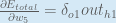
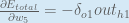
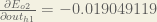
Finally, how much does the total net input of $o1$ change with respect to $w_5$ ?

$net_{o1} = w_5 * out_{h1} + w_6 * out_{h2} + b_2 * 1$

$\frac{\partial net_{o1}}{\partial w_{5}} = 1 * out_{h1} * w_5^{(1 - 1)} + 0 + 0 = out_{h1} = 0.593269992$

Putting it all together:

$\frac{\partial E_{total}}{\partial w_{5}} = \frac{\partial E_{total}}{\partial out_{o1}} * \frac{\partial out_{o1}}{\partial net_{o1}} * \frac{\partial net_{o1}}{\partial w_{5}}$

$\frac{\partial E_{total}}{\partial w_{5}} = 0.74136507 * 0.186815602 * 0.593269992 = 0.082167041$

You’ll often see this calculation combined in the form of the delta rule:

$\frac{\partial E_{total}}{\partial w_{5}} = -(target_{o1} - out_{o1}) * out_{o1}(1 - out_{o1}) * out_{h1}$

Alternatively, we have $\frac{\partial E_{total}}{\partial out_{o1}}$ and $\frac{\partial out_{o1}}{\partial net_{o1}}$ which can be written as $\frac{\partial E_{total}}{\partial net_{o1}}$ , aka $\delta_{o1}$ (the Greek letter delta) aka the node delta. We can use this to rewrite the calculation above:

$\delta_{o1} = \frac{\partial E_{total}}{\partial out_{o1}} * \frac{\partial out_{o1}}{\partial net_{o1}} = \frac{\partial E_{total}}{\partial net_{o1}}$

$\delta_{o1} = -(target_{o1} - out_{o1}) * out_{o1}(1 - out_{o1})$

Therefore:

$\frac{\partial E_{total}}{\partial w_{5}} = \delta_{o1} out_{h1}$

Some sources extract the negative sign from $\delta$ so it would be written as:

$\frac{\partial E_{total}}{\partial w_{5}} = -\delta_{o1} out_{h1}$

To decrease the error, we then subtract this value from the current weight (optionally multiplied by some learning rate, eta, which we’ll set to 0.5):

$w_5^{+} = w_5 - \eta * \frac{\partial E_{total}}{\partial w_{5}} = 0.4 - 0.5 * 0.082167041 = 0.35891648$

Some sources use $\alpha$ (alpha) to represent the learning rate, others use $\eta$ (eta), and others even use $\epsilon$ (epsilon).

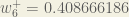
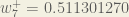
We can repeat this process to get the new weights $w_6$ , $w_7$ , and $w_8$ :

$w_6^{+} = 0.408666186$

$w_7^{+} = 0.511301270$

$w_8^{+} = 0.561370121$

We perform the actual updates in the neural network after we have the new weights leading into the hidden layer neurons (ie, we use the original weights, not the updated weights, when we continue the backpropagation algorithm below).

Hidden Layer

Next, we’ll continue the backwards pass by calculating new values for $w_1$ , $w_2$ , $w_3$ , and $w_4$ .

Big picture, here’s what we need to figure out:

$\frac{\partial E_{total}}{\partial w_{1}} = \frac{\partial E_{total}}{\partial out_{h1}} * \frac{\partial out_{h1}}{\partial net_{h1}} * \frac{\partial net_{h1}}{\partial w_{1}}$

Visually:

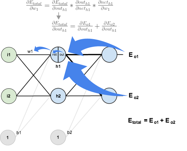
We’re going to use a similar process as we did for the output layer, but slightly different to account for the fact that the output of each hidden layer neuron contributes to the output (and therefore error) of multiple output neurons. We know that $out_{h1}$ affects both $out_{o1}$ and $out_{o2}$ therefore the $\frac{\partial E_{total}}{\partial out_{h1}}$ needs to take into consideration its effect on the both output neurons:

$\frac{\partial E_{total}}{\partial out_{h1}} = \frac{\partial E_{o1}}{\partial out_{h1}} + \frac{\partial E_{o2}}{\partial out_{h1}}$

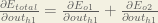
Starting with $\frac{\partial E_{o1}}{\partial out_{h1}}$ :

$\frac{\partial E_{o1}}{\partial out_{h1}} = \frac{\partial E_{o1}}{\partial net_{o1}} * \frac{\partial net_{o1}}{\partial out_{h1}}$

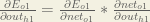
We can calculate $\frac{\partial E_{o1}}{\partial net_{o1}}$ using values we calculated earlier:

$\frac{\partial E_{o1}}{\partial net_{o1}} = \frac{\partial E_{o1}}{\partial out_{o1}} * \frac{\partial out_{o1}}{\partial net_{o1}} = 0.74136507 * 0.186815602 = 0.138498562$

And $\frac{\partial net_{o1}}{\partial out_{h1}}$ is equal to $w_5$ :

$net_{o1} = w_5 * out_{h1} + w_6 * out_{h2} + b_2 * 1$

$\frac{\partial net_{o1}}{\partial out_{h1}} = w_5 = 0.40$

Plugging them in:

$\frac{\partial E_{o1}}{\partial out_{h1}} = \frac{\partial E_{o1}}{\partial net_{o1}} * \frac{\partial net_{o1}}{\partial out_{h1}} = 0.138498562 * 0.40 = 0.055399425$

Following the same process for $\frac{\partial E_{o2}}{\partial out_{h1}}$ , we get:

$\frac{\partial E_{o2}}{\partial out_{h1}} = -0.019049119$

Therefore:

$\frac{\partial E_{total}}{\partial out_{h1}} = \frac{\partial E_{o1}}{\partial out_{h1}} + \frac{\partial E_{o2}}{\partial out_{h1}} = 0.055399425 + -0.019049119 = 0.036350306$

Now that we have $\frac{\partial E_{total}}{\partial out_{h1}}$ , we need to figure out $\frac{\partial out_{h1}}{\partial net_{h1}}$ and then $\frac{\partial net_{h1}}{\partial w}$ for each weight:

$out_{h1} = \frac{1}{1+e^{-net_{h1}}}$

$\frac{\partial out_{h1}}{\partial net_{h1}} = out_{h1}(1 - out_{h1}) = 0.59326999(1 - 0.59326999 ) = 0.241300709$

We calculate the partial derivative of the total net input to $h_1$ with respect to $w_1$ the same as we did for the output neuron:

$net_{h1} = w_1 * i_1 + w_3 * i_2 + b_1 * 1$

$\frac{\partial net_{h1}}{\partial w_1} = i_1 = 0.05$

Putting it all together:

$\frac{\partial E_{total}}{\partial w_{1}} = \frac{\partial E_{total}}{\partial out_{h1}} * \frac{\partial out_{h1}}{\partial net_{h1}} * \frac{\partial net_{h1}}{\partial w_{1}}$

$\frac{\partial E_{total}}{\partial w_{1}} = 0.036350306 * 0.241300709 * 0.05 = 0.000438568$

You might also see this written as:

$\frac{\partial E_{total}}{\partial w_{1}} = (\sum\limits_{o}{\frac{\partial E_{total}}{\partial out_{o}} * \frac{\partial out_{o}}{\partial net_{o}} * \frac{\partial net_{o}}{\partial out_{h1}}}) * \frac{\partial out_{h1}}{\partial net_{h1}} * \frac{\partial net_{h1}}{\partial w_{1}}$

$\frac{\partial E_{total}}{\partial w_{1}} = (\sum\limits_{o}{\delta_{o} * w_{ho}}) * out_{h1}(1 - out_{h1}) * i_{1}$

$\frac{\partial E_{total}}{\partial w_{1}} = \delta_{h1}i_{1}$

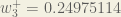
We can now update $w_1$ :

$w_1^{+} = w_1 - \eta * \frac{\partial E_{total}}{\partial w_{1}} = 0.15 - 0.5 * 0.000438568 = 0.149780716$

Repeating this for $w_2$ , $w_3$ , and $w_4$

$w_2^{+} = 0.19956143$

$w_3^{+} = 0.24975114$

$w_4^{+} = 0.29950229$

Finally, we’ve updated all of our weights! When we fed forward the 0.05 and 0.1 inputs originally, the error on the network was 0.298371109. After this first round of backpropagation, the total error is now down to 0.291027924. It might not seem like much, but after repeating this process 10,000 times, for example, the error plummets to 0.0000351085. At this point, when we feed forward 0.05 and 0.1, the two outputs neurons generate 0.015912196 (vs 0.01 target) and 0.984065734 (vs 0.99 target).

If you’ve made it this far and found any errors in any of the above or can think of any ways to make it clearer for future readers, don’t hesitate to drop me a note. Thanks!

1,006 thoughts on “A Step by Step Backpropagation Example”

Philippe Perez says:

September 24, 2021 at 12:47 pm

I think the formuale below is wrong. You should apply the multivariable version of the chaine rule instead.

\frac{\partial E_{total}}{\partial w_{5}} = \frac{\partial E_{total}}{\partial out_{o1}} * \frac{\partial out_{o1}}{\partial net_{o1}} * \frac{\partial net_{o1}}{\partial w_{5}}

Ingo Dahn says:

October 5, 2021 at 1:29 pm

Hi, it seems your network visualization is giving an error. numInputs not defined. Please, let me know when it is working, I’d like to check whether I can reference or include it into my materials.
Best
Ingo Dahn

com says:

December 4, 2021 at 5:25 pm

I’m assuming only one weight on the bias is just for simplicity?

- xmioviettel.net
Yoshiaki Fujita says:

December 12, 2021 at 11:51 pm

Thanks to such the nice explanation!
I implement my first neural network by referring the post, thanks.

Justin De Witt says:

December 16, 2021 at 1:06 pm

hello!

If there are multiple hidden layers, say two, three, or even more; How do you continue the back-propagation? Do you always take it two layers at a time?

If we are dealing with the leftmost hidden layer, do we need to track how changes to weights in this layer effect the following multiple hidden layers and then finally the output layer (working out error)

Tracing all routes that changes in a far left weight effect error seems to “blow up” very quickly so to speak.

Can anyone point me towards a worked example with at least 1 more hidden layer?

- Albrecht Ehlert says:
  
  December 20, 2021 at 11:48 am
  
  Hello Justin,
  the back-propagation works also with multiple hidden layers.
  You will find a good visualization for neural networks:
  http://playground.tensorflow.org/
  Sincerly
  Albrecht
  
Machine Learning Roadmap 2022 - Codelivly
DBM says:

December 29, 2021 at 6:49 am

Thank you for your detailed explanation.
I wonder how you set the outputs to be 0.01 and 0.99 ?
It is arbitrary chosen? Does the amount of the inputs and their vaules impact of the decesion how to set the outputs?