A Step by Step Backpropagation Example

March 17, 2015February 23, 2024Mazur

Background

Backpropagation is a common method for training a neural network. There is no shortage of papers online that attempt to explain how backpropagation works, but few that include an example with actual numbers. This post is my attempt to explain how it works with a concrete example that folks can compare their own calculations to in order to ensure they understand backpropagation correctly.

Backpropagation in Python

You can play around with a Python script that I wrote that implements the backpropagation algorithm in this Github repo.

Continue learning with Emergent Mind

If you find this tutorial useful and want to continue learning about AI/ML, I encourage you to check out Emergent Mind, a new website I’m working on that uses GPT-4 to surface and explain cutting-edge AI/ML papers:

In time, I hope to use AI to explain complex AI/ML topics on Emergent Mind in a style similar to what you’ll find in the tutorial below.

Now, on with the backpropagation tutorial…

Overview

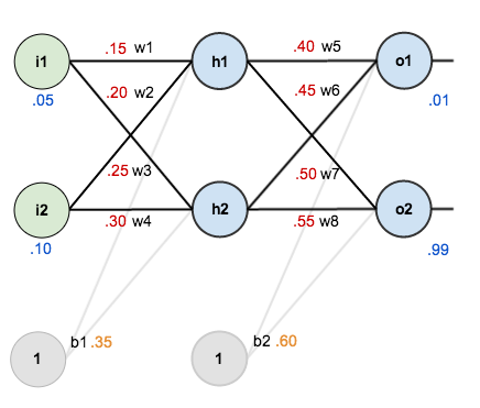
For this tutorial, we’re going to use a neural network with two inputs, two hidden neurons, two output neurons. Additionally, the hidden and output neurons will include a bias.

Here’s the basic structure:

In order to have some numbers to work with, here are the initial weights, the biases, and training inputs/outputs:

The goal of backpropagation is to optimize the weights so that the neural network can learn how to correctly map arbitrary inputs to outputs.

For the rest of this tutorial we’re going to work with a single training set: given inputs 0.05 and 0.10, we want the neural network to output 0.01 and 0.99.

The Forward Pass

To begin, lets see what the neural network currently predicts given the weights and biases above and inputs of 0.05 and 0.10. To do this we’ll feed those inputs forward though the network.

We figure out the total net input to each hidden layer neuron, squash the total net input using an activation function (here we use the logistic function), then repeat the process with the output layer neurons.

Total net input is also referred to as just net input by some sources.

Here’s how we calculate the total net input for $h_1$ :

$net_{h1} = w_1 * i_1 + w_2 * i_2 + b_1 * 1$

$net_{h1} = 0.15 * 0.05 + 0.2 * 0.1 + 0.35 * 1 = 0.3775$

We then squash it using the logistic function to get the output of $h_1$ :

$out_{h1} = \frac{1}{1+e^{-net_{h1}}} = \frac{1}{1+e^{-0.3775}} = 0.593269992$

Carrying out the same process for $h_2$ we get:

$out_{h2} = 0.596884378$

We repeat this process for the output layer neurons, using the output from the hidden layer neurons as inputs.

Here’s the output for $o_1$ :

$net_{o1} = w_5 * out_{h1} + w_6 * out_{h2} + b_2 * 1$

$net_{o1} = 0.4 * 0.593269992 + 0.45 * 0.596884378 + 0.6 * 1 = 1.105905967$

$out_{o1} = \frac{1}{1+e^{-net_{o1}}} = \frac{1}{1+e^{-1.105905967}} = 0.75136507$

And carrying out the same process for $o_2$ we get:

$out_{o2} = 0.772928465$

Calculating the Total Error

We can now calculate the error for each output neuron using the squared error function and sum them to get the total error:

$E_{total} = \sum \frac{1}{2}(target - output)^{2}$

Some sources refer to the target as the ideal and the output as the actual.

The $\frac{1}{2}$ is included so that exponent is cancelled when we differentiate later on. The result is eventually multiplied by a learning rate anyway so it doesn’t matter that we introduce a constant here [1].

For example, the target output for $o_1$ is 0.01 but the neural network output 0.75136507, therefore its error is:

$E_{o1} = \frac{1}{2}(target_{o1} - out_{o1})^{2} = \frac{1}{2}(0.01 - 0.75136507)^{2} = 0.274811083$

Repeating this process for $o_2$ (remembering that the target is 0.99) we get:

$E_{o2} = 0.023560026$

The total error for the neural network is the sum of these errors:

$E_{total} = E_{o1} + E_{o2} = 0.274811083 + 0.023560026 = 0.298371109$

The Backwards Pass

Our goal with backpropagation is to update each of the weights in the network so that they cause the actual output to be closer the target output, thereby minimizing the error for each output neuron and the network as a whole.

Output Layer

Consider $w_5$ . We want to know how much a change in $w_5$ affects the total error, aka $\frac{\partial E_{total}}{\partial w_{5}}$ .

$\frac{\partial E_{total}}{\partial w_{5}}$ is read as “the partial derivative of $E_{total}$ with respect to $w_{5}$ “. You can also say “the gradient with respect to $w_{5}$ ”.

By applying the chain rule we know that:

$\frac{\partial E_{total}}{\partial w_{5}} = \frac{\partial E_{total}}{\partial out_{o1}} * \frac{\partial out_{o1}}{\partial net_{o1}} * \frac{\partial net_{o1}}{\partial w_{5}}$

Visually, here’s what we’re doing:

We need to figure out each piece in this equation.

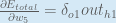
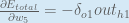
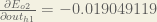
First, how much does the total error change with respect to the output?

$E_{total} = \frac{1}{2}(target_{o1} - out_{o1})^{2} + \frac{1}{2}(target_{o2} - out_{o2})^{2}$

$\frac{\partial E_{total}}{\partial out_{o1}} = 2 * \frac{1}{2}(target_{o1} - out_{o1})^{2 - 1} * -1 + 0$

$\frac{\partial E_{total}}{\partial out_{o1}} = -(target_{o1} - out_{o1}) = -(0.01 - 0.75136507) = 0.74136507$

$-(target - out)$ is sometimes expressed as $out - target$

When we take the partial derivative of the total error with respect to $out_{o1}$ , the quantity $\frac{1}{2}(target_{o2} - out_{o2})^{2}$ becomes zero because $out_{o1}$ does not affect it which means we’re taking the derivative of a constant which is zero.

Next, how much does the output of $o_1$ change with respect to its total net input?

The partial derivative of the logistic function is the output multiplied by 1 minus the output:

$out_{o1} = \frac{1}{1+e^{-net_{o1}}}$

$\frac{\partial out_{o1}}{\partial net_{o1}} = out_{o1}(1 - out_{o1}) = 0.75136507(1 - 0.75136507) = 0.186815602$

Finally, how much does the total net input of $o1$ change with respect to $w_5$ ?

$net_{o1} = w_5 * out_{h1} + w_6 * out_{h2} + b_2 * 1$

$\frac{\partial net_{o1}}{\partial w_{5}} = 1 * out_{h1} * w_5^{(1 - 1)} + 0 + 0 = out_{h1} = 0.593269992$

Putting it all together:

$\frac{\partial E_{total}}{\partial w_{5}} = \frac{\partial E_{total}}{\partial out_{o1}} * \frac{\partial out_{o1}}{\partial net_{o1}} * \frac{\partial net_{o1}}{\partial w_{5}}$

$\frac{\partial E_{total}}{\partial w_{5}} = 0.74136507 * 0.186815602 * 0.593269992 = 0.082167041$

You’ll often see this calculation combined in the form of the delta rule:

$\frac{\partial E_{total}}{\partial w_{5}} = -(target_{o1} - out_{o1}) * out_{o1}(1 - out_{o1}) * out_{h1}$

Alternatively, we have $\frac{\partial E_{total}}{\partial out_{o1}}$ and $\frac{\partial out_{o1}}{\partial net_{o1}}$ which can be written as $\frac{\partial E_{total}}{\partial net_{o1}}$ , aka $\delta_{o1}$ (the Greek letter delta) aka the node delta. We can use this to rewrite the calculation above:

$\delta_{o1} = \frac{\partial E_{total}}{\partial out_{o1}} * \frac{\partial out_{o1}}{\partial net_{o1}} = \frac{\partial E_{total}}{\partial net_{o1}}$

$\delta_{o1} = -(target_{o1} - out_{o1}) * out_{o1}(1 - out_{o1})$

Therefore:

$\frac{\partial E_{total}}{\partial w_{5}} = \delta_{o1} out_{h1}$

Some sources extract the negative sign from $\delta$ so it would be written as:

$\frac{\partial E_{total}}{\partial w_{5}} = -\delta_{o1} out_{h1}$

To decrease the error, we then subtract this value from the current weight (optionally multiplied by some learning rate, eta, which we’ll set to 0.5):

$w_5^{+} = w_5 - \eta * \frac{\partial E_{total}}{\partial w_{5}} = 0.4 - 0.5 * 0.082167041 = 0.35891648$

Some sources use $\alpha$ (alpha) to represent the learning rate, others use $\eta$ (eta), and others even use $\epsilon$ (epsilon).

We can repeat this process to get the new weights $w_6$ , $w_7$ , and $w_8$ :

$w_6^{+} = 0.408666186$

$w_7^{+} = 0.511301270$

$w_8^{+} = 0.561370121$

We perform the actual updates in the neural network after we have the new weights leading into the hidden layer neurons (ie, we use the original weights, not the updated weights, when we continue the backpropagation algorithm below).

Hidden Layer

Next, we’ll continue the backwards pass by calculating new values for $w_1$ , $w_2$ , $w_3$ , and $w_4$ .

Big picture, here’s what we need to figure out:

$\frac{\partial E_{total}}{\partial w_{1}} = \frac{\partial E_{total}}{\partial out_{h1}} * \frac{\partial out_{h1}}{\partial net_{h1}} * \frac{\partial net_{h1}}{\partial w_{1}}$

Visually:

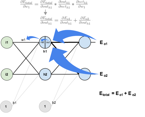
We’re going to use a similar process as we did for the output layer, but slightly different to account for the fact that the output of each hidden layer neuron contributes to the output (and therefore error) of multiple output neurons. We know that $out_{h1}$ affects both $out_{o1}$ and $out_{o2}$ therefore the $\frac{\partial E_{total}}{\partial out_{h1}}$ needs to take into consideration its effect on the both output neurons:

$\frac{\partial E_{total}}{\partial out_{h1}} = \frac{\partial E_{o1}}{\partial out_{h1}} + \frac{\partial E_{o2}}{\partial out_{h1}}$

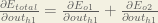
Starting with $\frac{\partial E_{o1}}{\partial out_{h1}}$ :

$\frac{\partial E_{o1}}{\partial out_{h1}} = \frac{\partial E_{o1}}{\partial net_{o1}} * \frac{\partial net_{o1}}{\partial out_{h1}}$

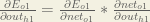
We can calculate $\frac{\partial E_{o1}}{\partial net_{o1}}$ using values we calculated earlier:

$\frac{\partial E_{o1}}{\partial net_{o1}} = \frac{\partial E_{o1}}{\partial out_{o1}} * \frac{\partial out_{o1}}{\partial net_{o1}} = 0.74136507 * 0.186815602 = 0.138498562$

And $\frac{\partial net_{o1}}{\partial out_{h1}}$ is equal to $w_5$ :

$net_{o1} = w_5 * out_{h1} + w_6 * out_{h2} + b_2 * 1$

$\frac{\partial net_{o1}}{\partial out_{h1}} = w_5 = 0.40$

Plugging them in:

$\frac{\partial E_{o1}}{\partial out_{h1}} = \frac{\partial E_{o1}}{\partial net_{o1}} * \frac{\partial net_{o1}}{\partial out_{h1}} = 0.138498562 * 0.40 = 0.055399425$

Following the same process for $\frac{\partial E_{o2}}{\partial out_{h1}}$ , we get:

$\frac{\partial E_{o2}}{\partial out_{h1}} = -0.019049119$

Therefore:

$\frac{\partial E_{total}}{\partial out_{h1}} = \frac{\partial E_{o1}}{\partial out_{h1}} + \frac{\partial E_{o2}}{\partial out_{h1}} = 0.055399425 + -0.019049119 = 0.036350306$

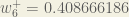
Now that we have $\frac{\partial E_{total}}{\partial out_{h1}}$ , we need to figure out $\frac{\partial out_{h1}}{\partial net_{h1}}$ and then $\frac{\partial net_{h1}}{\partial w}$ for each weight:

$out_{h1} = \frac{1}{1+e^{-net_{h1}}}$

$\frac{\partial out_{h1}}{\partial net_{h1}} = out_{h1}(1 - out_{h1}) = 0.59326999(1 - 0.59326999 ) = 0.241300709$

We calculate the partial derivative of the total net input to $h_1$ with respect to $w_1$ the same as we did for the output neuron:

$net_{h1} = w_1 * i_1 + w_3 * i_2 + b_1 * 1$

$\frac{\partial net_{h1}}{\partial w_1} = i_1 = 0.05$

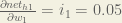
Putting it all together:

$\frac{\partial E_{total}}{\partial w_{1}} = \frac{\partial E_{total}}{\partial out_{h1}} * \frac{\partial out_{h1}}{\partial net_{h1}} * \frac{\partial net_{h1}}{\partial w_{1}}$

$\frac{\partial E_{total}}{\partial w_{1}} = 0.036350306 * 0.241300709 * 0.05 = 0.000438568$

You might also see this written as:

$\frac{\partial E_{total}}{\partial w_{1}} = (\sum\limits_{o}{\frac{\partial E_{total}}{\partial out_{o}} * \frac{\partial out_{o}}{\partial net_{o}} * \frac{\partial net_{o}}{\partial out_{h1}}}) * \frac{\partial out_{h1}}{\partial net_{h1}} * \frac{\partial net_{h1}}{\partial w_{1}}$

$\frac{\partial E_{total}}{\partial w_{1}} = (\sum\limits_{o}{\delta_{o} * w_{ho}}) * out_{h1}(1 - out_{h1}) * i_{1}$

$\frac{\partial E_{total}}{\partial w_{1}} = \delta_{h1}i_{1}$

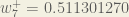
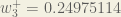
We can now update $w_1$ :

$w_1^{+} = w_1 - \eta * \frac{\partial E_{total}}{\partial w_{1}} = 0.15 - 0.5 * 0.000438568 = 0.149780716$

Repeating this for $w_2$ , $w_3$ , and $w_4$

$w_2^{+} = 0.19956143$

$w_3^{+} = 0.24975114$

$w_4^{+} = 0.29950229$

Finally, we’ve updated all of our weights! When we fed forward the 0.05 and 0.1 inputs originally, the error on the network was 0.298371109. After this first round of backpropagation, the total error is now down to 0.291027924. It might not seem like much, but after repeating this process 10,000 times, for example, the error plummets to 0.0000351085. At this point, when we feed forward 0.05 and 0.1, the two outputs neurons generate 0.015912196 (vs 0.01 target) and 0.984065734 (vs 0.99 target).

If you’ve made it this far and found any errors in any of the above or can think of any ways to make it clearer for future readers, don’t hesitate to drop me a note. Thanks!

And while I have you…

Again, if you liked this tutorial, please check out Emergent Mind, a site I’m building with an end goal of explaining AI/ML concepts in a similar style as this post. Feedback very much welcome!

1,111 thoughts on “A Step by Step Backpropagation Example”

Kwick says:

July 17, 2017 at 11:04 am

This example single handedly taught me how to actually make a neural network. My one question though pertains to the weights of the bias for each layer.
Are the bias’ and the bias weights supposed to remain unchanged, or are the weights adjusted through back propagation just as any other?

Reply
Jason says:

July 18, 2017 at 4:58 am

Hi,

Could you please explain why the biases are not get updated?

Reply
1. Apurwa says:
  
  July 25, 2017 at 12:19 pm
  
  That’s because the biases are threshold values that are by default set as constant (Their values are governed, depending on the application of NN, by one of the following : business logic, scientific fact such as 273Kelvin or 3*10^8m/s etc.)
  
  Reply
Vic Cassale says:

July 18, 2017 at 1:19 pm

Trying to understand why a multiplication with -1 in the dE(total)/dOut(o1).

if f(x) = a*x^r then

df(x) = r*a*x^(r-1)

in this particular case

f(x) = 1/2 * x ^ 2

df(x) = 2 * 1/2 * x ^ (2-1) = x

So dE(total)/dOut(o1) should be = target-actual

However, you are multiplying by -1 which makes it actual – target.

Where does the -1 come from?

Reply
1. Vic Cassale says:
  
  July 18, 2017 at 1:24 pm
  
  never mind, I just realized the x = actual and not target-actual so the -1 is (0-actual). It was just not very intuitive the way you wrote it. Maybe it’s worth adding an explanation…
  
  Reply
  1. Tim Thompson says:
    
    November 26, 2017 at 10:13 pm
    
    I agree, I was tripped up by this and am still having trouble with it. Vic, could you give a further example of how you understood it?
    
    Reply
2. Josimar Chire says:
  
  September 5, 2017 at 2:34 pm
  
  You must remind chain rule for derivatives.
  f'(x) = f'(x)x’
  
  Reply
  1. __Chris says:
    
    September 8, 2017 at 9:14 am
    
    could you explain it, I still dont know wheres does -1 come from :/
    
    Reply
    1. __Chris says:
      
      September 8, 2017 at 9:21 am
      
      ow ok, d(0.1) – d(out1) = 0 – 1
      
      Reply
Craig Matthews says:

July 19, 2017 at 9:08 am

Thank you so much. This helped tremendously!

Reply
Ivan Felipe Rodríguez says:

July 19, 2017 at 11:11 am

Great post! Thank you. I got a lot of insight on how backpropagation works.

Reply
Kimman says:

July 21, 2017 at 9:04 am

Excellent explanation

Reply
Gurpreet Mohaar says:

July 24, 2017 at 12:44 pm

This is excellent explanation.

Reply
Damien Hoffschir says:

July 25, 2017 at 5:57 am

Thank you, you helped me a lot.

I was working with Neural Networks – A Comprehensive Foundation by Simon Haykin. But Matt explanations are easier to work with.

Reply
J W says:

July 25, 2017 at 9:34 am

Fantastic. Greatly appreciated

Reply
Asher says:

July 25, 2017 at 10:11 pm

Great explanation deserves spreading!

Reply
adityapatgaonkar9 says:

July 27, 2017 at 3:21 am

Amazing explanation! Thanks for taking the effort!

Reply
Mikkel says:

July 28, 2017 at 10:55 am

Thanks for this!

Reply
Omnomonm says:

July 29, 2017 at 2:27 am

This helped me quite a bit, it explain back prop with a larger network, though there aren’t any numbers: https://cookedsashimi.wordpress.com/2017/05/06/an-example-of-backpropagation-in-a-four-layer-neural-network-using-cross-entropy-loss/?frame-nonce=f08dbcf84b

Reply
Kalin Dumitrescu says:

August 1, 2017 at 3:30 am

so how would the backpropagation look in the case of more hidden layers? for instance, if we have 2 hidden layers (1st layer with 2 neurons, second layer with 3), 2 input neurons and 2 output neurons. we want to find dEtotal/dw1. Would you have partial errors for each neuron in the second hidden layer? like dEh3/dneth3*w5+dEh4/dneth4*w7+dEh5/dneth5*w9 ? if so what is the value of each Ehx (x=3 to 5) or just how do you solve dEtotal/dw1?hope it makes sense

Reply
Pingback: 2. MNIST FOR ML BEGINNER – 아파트가 너무 비싸
justaminute says:

August 3, 2017 at 6:06 am

Your explanation was so helpful. The penny finally dropped. Thank you.

Reply
mt says:

August 4, 2017 at 9:22 am

It helped me a lot for creating my first neural network example. If you have difficulties for implementing your neural network.
Check my example : https://github.com/mlhtnc/deep-learning-example

Reply
1. Josimar says:
  
  September 9, 2017 at 1:52 am
  
  I have compiled your code and it’s working.
  
  Reply
asad says:

August 4, 2017 at 2:45 pm

Thanks a lot for clear explanation

Reply
Ha says:

August 7, 2017 at 1:51 pm

Do any body know any source to find a general equations for the feed forward back propagation. So we can apply the model for any number of hidden layers and output layers

Reply
Armando says:

August 14, 2017 at 3:50 am

Awesome! This post finally help me to code a learning layer only using a matrix library. I am a lazy tweeter but this totally deserves it. Even my source code has a link to this article! https://twitter.com/Corlaez/status/897002103478071297

Reply
Pingback: How to create a Neural Network in JavaScript in only 30 lines of code – Bit Treat
Tracy-G says:

August 19, 2017 at 12:12 pm

Matt, What if any is the relationship between your article (nice one just to add) and this YouTube video I found https://www.youtube.com/watch?v=xJkUKKxeYYg? There appears to be a lot in common.

Reply
helina says:

August 21, 2017 at 11:44 pm

Thank you so much, Matt! It`s the easiest explanation of backprop I have ever come across!

Reply
Joan says:

August 24, 2017 at 8:22 am

is this a right answer: w1..w8
-0,860918581,-1,807310582,-0,756487191,-1,69622177
-4,934133883,-4,808773679,3,736390466,3,738422962
Error=2,80447E-09
am I right?

Reply
abhilash reddy says:

August 28, 2017 at 1:04 am

Thankyo very much .I have been stumbling around many blogs to see how numerically back propagation work . You blog saved my time . :-)

Reply
spzhang says:

August 28, 2017 at 11:59 pm

Thanks for this valuable article. I have a equation. When you update the hidden layers, the following equation seems to be not correct.

\frac{\partial E_{o1}}{\partial out_{h1}} = \frac{\partial E_{o1}}{\partial net_{o1}} * \frac{\partial net_{o1}}{\partial out_{h1}}

Reply
1. Boaz Shvartzman says:
  
  October 3, 2017 at 11:19 am
  
  I noticed it too. The net_{o1} and out_{h1} should switch
  
  Reply
2. boaz85 says:
  
  October 3, 2017 at 11:21 am
  
  I noticed that too. net_{o1} and out_{o1} should be switched
  
  Reply
purna mallepaddi says:

September 1, 2017 at 4:42 am

awesome article to understand this crazy neural network stuff

Reply
Omar Elgazzar says:

September 2, 2017 at 1:10 am

I’m a beginner in ML. But I’ve learnt that the error function used with logistic (sigmoid) function isn’t convex, So we cannot use gradient descent algorithm due to local optima. So, why did we used it here?

Reply
1. Sai says:
  
  September 25, 2017 at 12:14 pm
  
  i guess we can still use it. It will converge to local optima. Global optima not guarenteed
  
  Reply
Pingback: What's the difference between reinforcement Learning and Deep-learning? | Eventwards
Xianglong says:

September 6, 2017 at 10:08 am

Many thanks! This is quite clear in mathematics and functionality.

Reply
Rachna K says:

September 7, 2017 at 3:58 am

Really Really helpful for understanding and visualising back-propagation. Beautifully explained and very nicely graphically shown too. Thanks a lot :D

Reply
Miftah says:

September 8, 2017 at 3:49 am

Good and informative post .One comment, the use of symbols in the diagram and the in the paragraphs where you explain the back prop steps are not similar(or I should say a bit different), it will be great if the same symbol can be used,

Reply
punyaswaroop12 says:

September 8, 2017 at 3:22 pm

Reblogged this on Algo Trading.

Reply
Sven says:

September 10, 2017 at 8:14 pm

hi, thank you very much, it ist simplest explanation I found about backprop in net. I could understand all your calculation up to the last point, where you say “After this first round of backpropagation, the total error is now down to 0.291027924”.
how did you come to this number? I think you did new forward pass with new weights and calculated new total error. do i see correct?

Reply
vladimirchebotarev says:

September 13, 2017 at 7:05 am

Thank you very much Matt, it greatly helped me to find the bug in my code. But your final values are not correct: it should be { 0.011587, 0.988459 } if you did not count first run and { 0.011587, 0.988458 } if you did.

Reply
alain boutin says:

September 14, 2017 at 12:03 pm

fantastically simple, i understand now !

Reply
Simon says:

September 16, 2017 at 9:00 am

Really great post, I love how you use the blue blocks to denote the different notation syntaxes of different sources. Very clear!

Reply
Prashant says:

September 17, 2017 at 8:25 am

You are GOD.I was stuck in week5 of Machine Learning course by Andrew.

Reply
Prashant says:

September 17, 2017 at 8:26 am

This comment section should be at top…

Reply
Prashant says:

September 17, 2017 at 11:39 am

Even noting and understanding from your blog took 3 hrs ,I am imagining how much time you would have devoted :)

Reply
gremberg2 says:

September 19, 2017 at 9:05 am

Danke!

Reply
Pingback: Some sites I found helpful in reviewing backprop – Into DL and Beyond
Pingback: My First Neural Net – Overthink
Pingback: BP神经网络 | Codeba
Atinesh says:

September 25, 2017 at 8:50 am

Thanks for such a clear explanation of backprop

Reply
ZR says:

September 30, 2017 at 9:24 am

Wonderful tutorial. I have a question with the initial calculation in the forward propagation. The calculation performed above states that the input for h1 is (0.15 * 0.05) + (0.2 * 0.1)+bias (weights 1 & 2). However, the graph, I think, shows (0.15 * 0.05) + (0.25 * 0.1)+bias (weights 1 & 3).

Have I looked at the graph incorrectly?

Thanks!

Reply
1. mrachid says:
  
  October 7, 2017 at 8:32 am
  
  If you look at the first graph, the one without the weight values, you can see that w1 and w2 is weights for h1 and that w3 and w4 are weights for h2. The graph with the values may make us mix up w2 and w3, because of the labels disposition.
  
  Reply
  1. mrachid says:
    
    October 7, 2017 at 8:33 am
    
    Great tutorial, btw :)
    
    Reply
Laurent A. says:

October 4, 2017 at 3:22 pm

I have found here an explanation on why the gradient for the output layer was simply “output – target”. Now, I got it. 1000 thanks for taking time to share :)

Reply
Vinay says:

October 6, 2017 at 8:56 am

Very good explanation with nice example. Thank you very much!!!

Reply
Pingback: A Deep Learning primer for all » Prithiviraj Damodaran
Anusha says:

October 8, 2017 at 8:52 pm

Thnaks a ton for such a crystal clear explanation! Made my day :)

Reply