A Step by Step Backpropagation Example

March 17, 2015February 23, 2024Mazur

Background

Backpropagation is a common method for training a neural network. There is no shortage of papers online that attempt to explain how backpropagation works, but few that include an example with actual numbers. This post is my attempt to explain how it works with a concrete example that folks can compare their own calculations to in order to ensure they understand backpropagation correctly.

Backpropagation in Python

You can play around with a Python script that I wrote that implements the backpropagation algorithm in this Github repo.

Continue learning with Emergent Mind

If you find this tutorial useful and want to continue learning about AI/ML, I encourage you to check out Emergent Mind, a new website I’m working on that uses GPT-4 to surface and explain cutting-edge AI/ML papers:

In time, I hope to use AI to explain complex AI/ML topics on Emergent Mind in a style similar to what you’ll find in the tutorial below.

Now, on with the backpropagation tutorial…

Overview

For this tutorial, we’re going to use a neural network with two inputs, two hidden neurons, two output neurons. Additionally, the hidden and output neurons will include a bias.

Here’s the basic structure:

In order to have some numbers to work with, here are the initial weights, the biases, and training inputs/outputs:

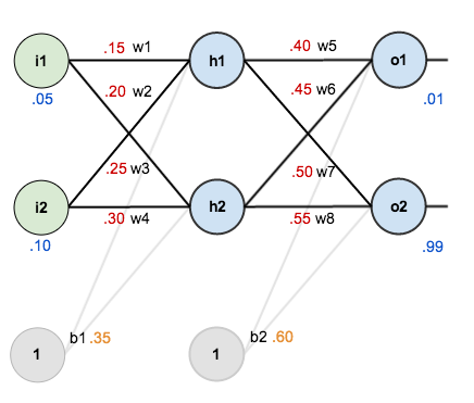
The goal of backpropagation is to optimize the weights so that the neural network can learn how to correctly map arbitrary inputs to outputs.

For the rest of this tutorial we’re going to work with a single training set: given inputs 0.05 and 0.10, we want the neural network to output 0.01 and 0.99.

The Forward Pass

To begin, lets see what the neural network currently predicts given the weights and biases above and inputs of 0.05 and 0.10. To do this we’ll feed those inputs forward though the network.

We figure out the total net input to each hidden layer neuron, squash the total net input using an activation function (here we use the logistic function), then repeat the process with the output layer neurons.

Total net input is also referred to as just net input by some sources.

Here’s how we calculate the total net input for $h_1$ :

$net_{h1} = w_1 * i_1 + w_2 * i_2 + b_1 * 1$

$net_{h1} = 0.15 * 0.05 + 0.2 * 0.1 + 0.35 * 1 = 0.3775$

We then squash it using the logistic function to get the output of $h_1$ :

$out_{h1} = \frac{1}{1+e^{-net_{h1}}} = \frac{1}{1+e^{-0.3775}} = 0.593269992$

Carrying out the same process for $h_2$ we get:

$out_{h2} = 0.596884378$

We repeat this process for the output layer neurons, using the output from the hidden layer neurons as inputs.

Here’s the output for $o_1$ :

$net_{o1} = w_5 * out_{h1} + w_6 * out_{h2} + b_2 * 1$

$net_{o1} = 0.4 * 0.593269992 + 0.45 * 0.596884378 + 0.6 * 1 = 1.105905967$

$out_{o1} = \frac{1}{1+e^{-net_{o1}}} = \frac{1}{1+e^{-1.105905967}} = 0.75136507$

And carrying out the same process for $o_2$ we get:

$out_{o2} = 0.772928465$

Calculating the Total Error

We can now calculate the error for each output neuron using the squared error function and sum them to get the total error:

$E_{total} = \sum \frac{1}{2}(target - output)^{2}$

Some sources refer to the target as the ideal and the output as the actual.

The $\frac{1}{2}$ is included so that exponent is cancelled when we differentiate later on. The result is eventually multiplied by a learning rate anyway so it doesn’t matter that we introduce a constant here [1].

For example, the target output for $o_1$ is 0.01 but the neural network output 0.75136507, therefore its error is:

$E_{o1} = \frac{1}{2}(target_{o1} - out_{o1})^{2} = \frac{1}{2}(0.01 - 0.75136507)^{2} = 0.274811083$

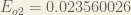
Repeating this process for $o_2$ (remembering that the target is 0.99) we get:

$E_{o2} = 0.023560026$

The total error for the neural network is the sum of these errors:

$E_{total} = E_{o1} + E_{o2} = 0.274811083 + 0.023560026 = 0.298371109$

The Backwards Pass

Our goal with backpropagation is to update each of the weights in the network so that they cause the actual output to be closer the target output, thereby minimizing the error for each output neuron and the network as a whole.

Output Layer

Consider $w_5$ . We want to know how much a change in $w_5$ affects the total error, aka $\frac{\partial E_{total}}{\partial w_{5}}$ .

$\frac{\partial E_{total}}{\partial w_{5}}$ is read as “the partial derivative of $E_{total}$ with respect to $w_{5}$ “. You can also say “the gradient with respect to $w_{5}$ ”.

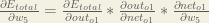
By applying the chain rule we know that:

$\frac{\partial E_{total}}{\partial w_{5}} = \frac{\partial E_{total}}{\partial out_{o1}} * \frac{\partial out_{o1}}{\partial net_{o1}} * \frac{\partial net_{o1}}{\partial w_{5}}$

Visually, here’s what we’re doing:

We need to figure out each piece in this equation.

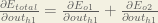
First, how much does the total error change with respect to the output?

$E_{total} = \frac{1}{2}(target_{o1} - out_{o1})^{2} + \frac{1}{2}(target_{o2} - out_{o2})^{2}$

$\frac{\partial E_{total}}{\partial out_{o1}} = 2 * \frac{1}{2}(target_{o1} - out_{o1})^{2 - 1} * -1 + 0$

$\frac{\partial E_{total}}{\partial out_{o1}} = -(target_{o1} - out_{o1}) = -(0.01 - 0.75136507) = 0.74136507$

$-(target - out)$ is sometimes expressed as $out - target$

When we take the partial derivative of the total error with respect to $out_{o1}$ , the quantity $\frac{1}{2}(target_{o2} - out_{o2})^{2}$ becomes zero because $out_{o1}$ does not affect it which means we’re taking the derivative of a constant which is zero.

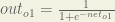
Next, how much does the output of $o_1$ change with respect to its total net input?

The partial derivative of the logistic function is the output multiplied by 1 minus the output:

$out_{o1} = \frac{1}{1+e^{-net_{o1}}}$

$\frac{\partial out_{o1}}{\partial net_{o1}} = out_{o1}(1 - out_{o1}) = 0.75136507(1 - 0.75136507) = 0.186815602$

Finally, how much does the total net input of $o1$ change with respect to $w_5$ ?

$net_{o1} = w_5 * out_{h1} + w_6 * out_{h2} + b_2 * 1$

$\frac{\partial net_{o1}}{\partial w_{5}} = 1 * out_{h1} * w_5^{(1 - 1)} + 0 + 0 = out_{h1} = 0.593269992$

Putting it all together:

$\frac{\partial E_{total}}{\partial w_{5}} = \frac{\partial E_{total}}{\partial out_{o1}} * \frac{\partial out_{o1}}{\partial net_{o1}} * \frac{\partial net_{o1}}{\partial w_{5}}$

$\frac{\partial E_{total}}{\partial w_{5}} = 0.74136507 * 0.186815602 * 0.593269992 = 0.082167041$

You’ll often see this calculation combined in the form of the delta rule:

$\frac{\partial E_{total}}{\partial w_{5}} = -(target_{o1} - out_{o1}) * out_{o1}(1 - out_{o1}) * out_{h1}$

Alternatively, we have $\frac{\partial E_{total}}{\partial out_{o1}}$ and $\frac{\partial out_{o1}}{\partial net_{o1}}$ which can be written as $\frac{\partial E_{total}}{\partial net_{o1}}$ , aka $\delta_{o1}$ (the Greek letter delta) aka the node delta. We can use this to rewrite the calculation above:

$\delta_{o1} = \frac{\partial E_{total}}{\partial out_{o1}} * \frac{\partial out_{o1}}{\partial net_{o1}} = \frac{\partial E_{total}}{\partial net_{o1}}$

$\delta_{o1} = -(target_{o1} - out_{o1}) * out_{o1}(1 - out_{o1})$

Therefore:

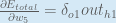
$\frac{\partial E_{total}}{\partial w_{5}} = \delta_{o1} out_{h1}$

Some sources extract the negative sign from $\delta$ so it would be written as:

$\frac{\partial E_{total}}{\partial w_{5}} = -\delta_{o1} out_{h1}$

To decrease the error, we then subtract this value from the current weight (optionally multiplied by some learning rate, eta, which we’ll set to 0.5):

$w_5^{+} = w_5 - \eta * \frac{\partial E_{total}}{\partial w_{5}} = 0.4 - 0.5 * 0.082167041 = 0.35891648$

Some sources use $\alpha$ (alpha) to represent the learning rate, others use $\eta$ (eta), and others even use $\epsilon$ (epsilon).

We can repeat this process to get the new weights $w_6$ , $w_7$ , and $w_8$ :

$w_6^{+} = 0.408666186$

$w_7^{+} = 0.511301270$

$w_8^{+} = 0.561370121$

We perform the actual updates in the neural network after we have the new weights leading into the hidden layer neurons (ie, we use the original weights, not the updated weights, when we continue the backpropagation algorithm below).

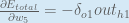
Hidden Layer

Next, we’ll continue the backwards pass by calculating new values for $w_1$ , $w_2$ , $w_3$ , and $w_4$ .

Big picture, here’s what we need to figure out:

$\frac{\partial E_{total}}{\partial w_{1}} = \frac{\partial E_{total}}{\partial out_{h1}} * \frac{\partial out_{h1}}{\partial net_{h1}} * \frac{\partial net_{h1}}{\partial w_{1}}$

Visually:

We’re going to use a similar process as we did for the output layer, but slightly different to account for the fact that the output of each hidden layer neuron contributes to the output (and therefore error) of multiple output neurons. We know that $out_{h1}$ affects both $out_{o1}$ and $out_{o2}$ therefore the $\frac{\partial E_{total}}{\partial out_{h1}}$ needs to take into consideration its effect on the both output neurons:

$\frac{\partial E_{total}}{\partial out_{h1}} = \frac{\partial E_{o1}}{\partial out_{h1}} + \frac{\partial E_{o2}}{\partial out_{h1}}$

Starting with $\frac{\partial E_{o1}}{\partial out_{h1}}$ :

$\frac{\partial E_{o1}}{\partial out_{h1}} = \frac{\partial E_{o1}}{\partial net_{o1}} * \frac{\partial net_{o1}}{\partial out_{h1}}$

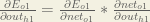
We can calculate $\frac{\partial E_{o1}}{\partial net_{o1}}$ using values we calculated earlier:

$\frac{\partial E_{o1}}{\partial net_{o1}} = \frac{\partial E_{o1}}{\partial out_{o1}} * \frac{\partial out_{o1}}{\partial net_{o1}} = 0.74136507 * 0.186815602 = 0.138498562$

And $\frac{\partial net_{o1}}{\partial out_{h1}}$ is equal to $w_5$ :

$net_{o1} = w_5 * out_{h1} + w_6 * out_{h2} + b_2 * 1$

$\frac{\partial net_{o1}}{\partial out_{h1}} = w_5 = 0.40$

Plugging them in:

$\frac{\partial E_{o1}}{\partial out_{h1}} = \frac{\partial E_{o1}}{\partial net_{o1}} * \frac{\partial net_{o1}}{\partial out_{h1}} = 0.138498562 * 0.40 = 0.055399425$

Following the same process for $\frac{\partial E_{o2}}{\partial out_{h1}}$ , we get:

$\frac{\partial E_{o2}}{\partial out_{h1}} = -0.019049119$

Therefore:

$\frac{\partial E_{total}}{\partial out_{h1}} = \frac{\partial E_{o1}}{\partial out_{h1}} + \frac{\partial E_{o2}}{\partial out_{h1}} = 0.055399425 + -0.019049119 = 0.036350306$

Now that we have $\frac{\partial E_{total}}{\partial out_{h1}}$ , we need to figure out $\frac{\partial out_{h1}}{\partial net_{h1}}$ and then $\frac{\partial net_{h1}}{\partial w}$ for each weight:

$out_{h1} = \frac{1}{1+e^{-net_{h1}}}$

$\frac{\partial out_{h1}}{\partial net_{h1}} = out_{h1}(1 - out_{h1}) = 0.59326999(1 - 0.59326999 ) = 0.241300709$

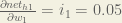
We calculate the partial derivative of the total net input to $h_1$ with respect to $w_1$ the same as we did for the output neuron:

$net_{h1} = w_1 * i_1 + w_3 * i_2 + b_1 * 1$

$\frac{\partial net_{h1}}{\partial w_1} = i_1 = 0.05$

Putting it all together:

$\frac{\partial E_{total}}{\partial w_{1}} = \frac{\partial E_{total}}{\partial out_{h1}} * \frac{\partial out_{h1}}{\partial net_{h1}} * \frac{\partial net_{h1}}{\partial w_{1}}$

$\frac{\partial E_{total}}{\partial w_{1}} = 0.036350306 * 0.241300709 * 0.05 = 0.000438568$

You might also see this written as:

$\frac{\partial E_{total}}{\partial w_{1}} = (\sum\limits_{o}{\frac{\partial E_{total}}{\partial out_{o}} * \frac{\partial out_{o}}{\partial net_{o}} * \frac{\partial net_{o}}{\partial out_{h1}}}) * \frac{\partial out_{h1}}{\partial net_{h1}} * \frac{\partial net_{h1}}{\partial w_{1}}$

$\frac{\partial E_{total}}{\partial w_{1}} = (\sum\limits_{o}{\delta_{o} * w_{ho}}) * out_{h1}(1 - out_{h1}) * i_{1}$

$\frac{\partial E_{total}}{\partial w_{1}} = \delta_{h1}i_{1}$

We can now update $w_1$ :

$w_1^{+} = w_1 - \eta * \frac{\partial E_{total}}{\partial w_{1}} = 0.15 - 0.5 * 0.000438568 = 0.149780716$

Repeating this for $w_2$ , $w_3$ , and $w_4$

$w_2^{+} = 0.19956143$

$w_3^{+} = 0.24975114$

$w_4^{+} = 0.29950229$

Finally, we’ve updated all of our weights! When we fed forward the 0.05 and 0.1 inputs originally, the error on the network was 0.298371109. After this first round of backpropagation, the total error is now down to 0.291027924. It might not seem like much, but after repeating this process 10,000 times, for example, the error plummets to 0.0000351085. At this point, when we feed forward 0.05 and 0.1, the two outputs neurons generate 0.015912196 (vs 0.01 target) and 0.984065734 (vs 0.99 target).

If you’ve made it this far and found any errors in any of the above or can think of any ways to make it clearer for future readers, don’t hesitate to drop me a note. Thanks!

And while I have you…

Again, if you liked this tutorial, please check out Emergent Mind, a site I’m building with an end goal of explaining AI/ML concepts in a similar style as this post. Feedback very much welcome!

1,090 thoughts on “A Step by Step Backpropagation Example”

Ilya Nonename says:

December 14, 2017 at 12:15 pm

Very, nice.
Did not succeed at first, because i was using 0 and 1 in one of inputs.
I figured out that 0 does not adjust weight.
So i shifted inputs by 0.5 (-0.5 and 0.5 instead 0 and 1) and it worked.

Reply
1. Aditya Mhatre says:
  
  February 21, 2018 at 4:01 pm
  
  That is precisely why biases are used.
  
  Reply
neuralnetwork963574777 says:

December 15, 2017 at 1:04 am

Hi Matt,
One question. In this article you calculate the Error function at the end of the forward propagation process as

E_{total} = \sum \frac{1}{2}(target – output)^{2}

I understand that this way of calculating the Error function was mostly used in the past and now we should use cross entropy. However, getting back to the squared error function – because the difference between the target and output is power 2, the result is always positive (regardless whether target > output or vice versa). That means that regardless that the actual network output result (target – output) can be positive error or negative error, we always back propagate the positive E function and eventually use the fractions of it at any neuron to adjust its weight and bias.
So, the adjustment goes always in one direction. Since it was successfully used in the past, how that worked? Or getting back to your example, we can use different input number and come up with negative (target – output) but the Error function will still be positive, and so the weight and bios adjustments for each neuron.

Regards
Igor

Reply
1. Henry Henri says:
  
  January 2, 2018 at 12:43 pm
  
  The squared error is always positive. But for backpropagation you use the (partial) derivative of the error function, which is linear and hence can be positive or negative.
  
  Reply
Wowza says:

December 17, 2017 at 11:28 pm

Man I’m studying for a final and this explained the algorithm better than the textbook. you’re actively the best

Reply
Shashank says:

December 18, 2017 at 1:00 pm

Amazing explanation!! can you please explain in the similar fashion about updating the bias. As i am confused bias is only for a layer how can we update for every neuron??

Reply
Vinicius Silva says:

December 18, 2017 at 6:23 pm

So what happens next? What do you mean by “after repeating this process 10,000 times, for example, the error plummets to 0.0000351085”? Should we keep using the same input record in all these 10000 iterations? I think I understood what has been explained by this text, but I wish you could ellaborate a bit more on the whole neural network learning process.

Also, can you provide a general idea on what is happening in your neural network visualization example? What were you feeding the network during all those many iterations?

Sorry for asking so many questions, it’s just I’m trying to get a deep understanding on this topic, but failing to find quality material that isn’t too difficult for beginner like me.

Thank you.

Reply
oliveiravini1994 says:

December 18, 2017 at 6:25 pm

So what happens next? What do you mean by “after repeating this process 10,000 times, for example, the error plummets to 0.0000351085”? Should we keep using the same input record in all these 10000 iterations? I think I understood what has been explained by this text, but I wish you could ellaborate a bit more on the whole neural network learning process.

Also, can you provide a general idea on what is happening in your neural network visualization example? What were you feeding the network during all those many iterations?

Sorry for asking so many questions, it’s just I’m trying to get a deep understanding on this topic, but failing to find quality material that isn’t too difficult for beginner like me.

Thank you.

Reply
1. Daniel says:
  
  December 23, 2017 at 10:18 pm
  
  this network doesn’t work well, my outputs are exactly like the example above, but training 16000 inputs for xor problem, the error is still very big, with another net I got very small error with 2000 inputs and i didnt even touch eta
  
  Reply
2. Henry Henri says:
  
  January 2, 2018 at 12:54 pm
  
  If I get your question correctly you’re asking, whether to keep using the same input for all training cycles, then the answer is no. The network learns by example. The more examples you show the more it will learn. If you only show one example, that’s the only case it will be able to work with. Depending on the complexity of the task you might need to teach tens of thousands of different samples throughout training. In some cases, it is appropriate to show the same sample multiple times. E.g. if you want to train XOR (you need at least one hidden layer for this) you have the possible samples (0,0 => 0) (1,0 => 1) (0,1 => 1) and (1,1 => 0). You run them in some random order until you have reached an error rate you’re comfortable with.
  
  Reply
Daniel says:

December 19, 2017 at 2:34 pm

why should it be called backpropagation if you don’t update the weights after you calculed them? you can easily perform this operation from the input layer to the output layer and get the same result… are you sure about “we use the original weights, not the updated weights, when we continue the backpropagation algorithm below” ?

Reply
1. Henry Henri says:
  
  January 2, 2018 at 12:47 pm
  
  Updating and backpropagation are two separate steps. Backpropagation pushes the error back through the network to find out how much responsibility to assign to each weight. This responsibility is then used to update the weights. You can interleave backpropagation and update for each layer, but first, you have to calculate the error for the next layer before you can do the update.
  
  Reply
Adam Girycki says:

December 20, 2017 at 1:24 pm

Great explanation! Short and clear!

Reply
WangLu says:

December 20, 2017 at 9:44 pm

Great simpification a NN to a two layer single data structure. It’s really easy to learn for beginner. Thanks man.

Reply
Daniel Zheng says:

December 23, 2017 at 10:10 pm

Great tutorial just finished going through the math and managed to reproduce the calculation. Only a matter of time until I master it.

Reply
rspurge2 says:

December 25, 2017 at 3:17 pm

This was seriously helpful. Thanks for writing it!

Reply
vinith kumar says:

December 28, 2017 at 12:22 am

why bias weight is not updated?

Reply
Saurabh says:

December 28, 2017 at 4:29 am

Simple and intuitive explanation !! This is what I was looking for. Thank you.

Reply
Wallen Tan says:

December 30, 2017 at 7:38 pm

Really good tutorial! One of the most helpful ones I’ve come across.

Does the bias unit in each layer have only one weight or would there be a separate weight per connection with the nodes?

Reply
Willy Wonka says:

January 2, 2018 at 9:43 am

Man you explained it all, i have finally succeeded to implement hidden layer backpropagation now. THANKS!

Reply
Henry Henri says:

January 2, 2018 at 12:49 pm

Maybe I missed it, but I think you left out the update of the biases. It’s simple but still might not be obvious to everyone new to the topic.

Reply
James Liu says:

January 4, 2018 at 1:49 am

hi, i have two questions:
1) how do u ensure differentiating give the minimum value? instead of giving the maximum value?
2) Won’t differentiating it once give the lowest maximum value? which is the smallest error. why do we have to differentiate it 10000 times?

thanks, from singapore here!

Reply
Priyank says:

January 4, 2018 at 11:38 am

Dear sir,
Error should be:
Error=(1/2)(out-target)^2
isn’t it?

Reply
1. Priyank says:
  
  January 4, 2018 at 11:54 am
  
  sorry it’s correct
  
  Reply
Rashmi G says:

January 8, 2018 at 5:26 am

Hi..A very useful article..I have a doubt with calculating error for o1 . Here I am getting a negative value (-0.2747). Kindly help me here. Thanks in advance.

Reply
Karim Fouad says:

January 8, 2018 at 10:17 am

Thank you for this great tutorial.

Reply
1. Karim Fouad says:
  
  January 8, 2018 at 10:20 am
  
  for those who ask about bias updating you may assume the weights of bias as W’ 1 , W’ 2 , W’ 3 , W’ 4 and then apply same process on them
  
  Reply
Pingback: Draft
Pingback: How To Build an Artificial Neural Network From Scratch
Deept says:

January 13, 2018 at 4:43 am

This is the best explanation of backward propagation I ever read.!!

Reply
Manas says:

January 17, 2018 at 9:49 pm

This is so far the best explanation of backprop I read so far. Thankyou so much for this!

Reply
felipe says:

January 18, 2018 at 2:39 pm

“We can calculate \frac{\partial E_{o1}}{\partial net_{o1}} using values we calculated earlier: ” whats going on here? how do i get the result?

Great explanation btw

Reply
Kashyap Mahanta says:

January 21, 2018 at 1:21 am

The best one so far !!!

Reply
Ankit Bhaukajee says:

January 25, 2018 at 9:54 am

This blog is the best of the best explanation I have found in decoding backprop. Everybody was giving their own formula and I was not able to grasp the intuition but this post really helped me what is happening inside. Thank you for helping people.

Reply
Thomas says:

January 28, 2018 at 1:41 pm

Amazing explanation!
Though I used some random inputs and set the target values to double the input values (so the first output of the network is double the value of the first input, and the second output is double the value of the second input). It worked perfectly for specific input values. For example [0.03,0.09] would output very close to [0.06,0.18].
Though when I ran the algorithm in a loop many times, then tested the network (i.e. without using backprop and target values) it just outputted the same values that were outputted in the last iteration of the loop, rather than doubling the new values I inputted into the network.
So basically it only worked when I ran the backprop with the target values – though I want it to work without the target values!
Can anyone suggest anything? Sorry if I’m not being very clear, I’d be happy to explain myself if anyone is confused about what I mean.

Reply
1. Thomas says:
  
  January 30, 2018 at 1:28 pm
  
  Don’t worry, I worked it out! I was backpropagating too much for each pair of inputs, and not putting enough test inputs in. I should’ve been backpropagating alot less and using alot more test inputs!
  
  Reply
Christophe Schnitzler says:

January 30, 2018 at 6:02 am

Hi
I really don’t get how you calculate this line
\frac{\partial E_{total}}{\partial out_{o1}} = 2 * \frac{1}{2}(target_{o1} – out_{o1})^{2 – 1} * -1 + 0
I’m sure it is really simple, but cannot figure it out. Thanks for your help!

Reply
1. Nabil says:
  
  February 2, 2018 at 7:05 am
  
  Yeah, im stuck at this part too. Cant figure it out..
  
  Reply
2. Kalin Stoyanov says:
  
  February 2, 2018 at 8:01 am
  
  That’s how you calculate the partial derivative:
  https://www.derivative-calculator.net/#expr=1%2F2%28x-y%29%5E2%20%2B%201%2F2%28z%2Bt%29%5E2&diffvar=y&showsteps=1
  
  Reply
3. Tsviatko Jongov says:
  
  February 20, 2018 at 4:14 am
  
  First you get derivative of the outer function, then you multiply by the derivative of the inner function (which results in -1). And finally the derivative of the second part of the equation is 0 since it considered as a constant.
  
  Reply
4. Luis Andres says:
  
  February 24, 2018 at 1:05 pm
  
  it is just the first derivative of the error.
  
  Reply
Pingback: Сверточная нейронная сеть, часть 2: обучение алгоритмом обратного распространения ошибки – CHEPA website
Pingback: Сверточная нейронная сеть, часть 2: обучение алгоритмом обратного распространения ошибки — Богданович Онлайн
Pingback: Сверточная нейронная сеть, часть 2: обучение алгоритмом обратного распространения ошибки | Компьюлента
Marius A says:

February 1, 2018 at 8:14 pm

Thanks for the great guide. I programmed a neural network based on this tutorial.
Here is a hint for programmers, so you can save some debugging time:
When calculating this value:
out_h1 * (out_h1 – 1)
out_h1 will sometimes be 1 if the sum of the inputs of a neuron is too high. You’ll end up with 0, which means you won’t update the weights.
Make sure to set this value to 0.0001 if it ends up being 0.

Reply
nick says:

February 4, 2018 at 3:15 am

hello, i think this step is not correct?
partial out1/partial net1 = out1*(1-out1)
should equal with: net1*(1-net1)?

Reply
joskid says:

February 5, 2018 at 10:46 am

Reblogged this on josephdung.

Reply
Louis says:

February 5, 2018 at 11:18 am

Do u have RNN bptt tutorial? That’s hard to know. Thx

Reply
Pingback: Building a Neural Network | Data Warehousing, BI and Data Science
Prabhat says:

February 7, 2018 at 7:15 pm

Simple amazing. Thanks a lot for a nice worked out example.

Reply
Gabriel M. says:

February 13, 2018 at 7:22 am

There is a mistake in the updated weights w6, w7
w6 = ~0.40891648
w7 = ~0.51137012

Reply
gabimuresan says:

February 13, 2018 at 7:24 am

There is a mistake in the calculations of w6 and w7
w6 = ~ 0.40891648
w7 = ~ 0.51137012

Reply
Matteo Costantini says:

February 14, 2018 at 7:12 am

Hi Matt, why when you take the partial derivative of the total error with respect to out1, you multiply by (-1)??
Thanks you

Reply
spamzero says:

February 14, 2018 at 9:39 pm

Read this post with this http://neuralnetworksanddeeplearning.com/chap2.html one together will help you get a better understanding of backpropagation.

Reply
Ymi Yugy says:

February 15, 2018 at 12:56 pm

Thanks. I think I finally got a grasp on backpropagstion. The only thing missing is the notation via vectors and matrices, but those shouldn’t be to difficult.

Reply
Lowell says:

February 15, 2018 at 2:41 pm

I rescind my previous agreement with Christophe. The -1 in the equation:

\frac{\partial E_{total}}{\partial out_{o1}} = 2 * \frac{1}{2}(target_{o1} – out_{o1})^{2 – 1} * -1 + 0

comes from the chain rule of differentiation. Which says: derivative of f(g) is

f'(g) * g’

In this case, we are taking the partial derivative with respect to out1, which makes f be 1/2(g)^2, with g being (target – out1). So the derivative is

1/2 * 2 * (target – out)^1 * -1

And the zero of course comes from the fact that those parts of the equation are not dependent on out1 at all and are thus constant with derivative zero.

Reply
Pingback: A ‘family-tree’ of words from a recurrent net – mind-builder's blog
Ben Fox says:

February 18, 2018 at 4:34 pm

Thank you! This is by far the best explanation on the topic I have seen. Is there any chance of adding a PrintFriendly/PDF link of this article? I would love to have this on my desk as a reference.

Reply
AJ says:

February 21, 2018 at 7:28 pm

You explained so nice, thank you so much!

Reply
Tosh Parsely says:

February 21, 2018 at 8:58 pm

How come when I run the XOR problem, the error I get never goes below < 0.50? Even after 5000 iterations, it keeps come out to be around .50.

Reply
Manuj Sharma says:

February 23, 2018 at 2:47 am

Very useful article. Thanks.

Reply
Ram Sethuraman says:

February 23, 2018 at 7:22 am

Hey. I think there is a problem with this explanation.
Shouldn’t d(E(total))/d(out h1) be equal to [d(E(total))/d(Eo1)* (d(Eo1)/d(out h1))] + [d(E(total))/d(Eo2)* (d(Eo2)/d(out h1))].

But it is given to be just (d(Eo1)/d(out h1) + (d(Eo2)/d(out h1)

Or am I wrong? Please help

Reply
1. Ashutosh Chandra says:
  
  April 15, 2018 at 2:29 pm
  
  Awesome tutorial. I really understood ” propagating the error backwards” concept for the first time.
  
  Reply