A Step by Step Backpropagation Example

Background

Backpropagation is a common method for training a neural network. There is no shortage of papers online that attempt to explain how backpropagation works, but few that include an example with actual numbers. This post is my attempt to explain how it works with a concrete example that folks can compare their own calculations to in order to ensure they understand backpropagation correctly.

Backpropagation in Python

You can play around with a Python script that I wrote that implements the backpropagation algorithm in this Github repo.

Backpropagation Visualization

For an interactive visualization showing a neural network as it learns, check out my Neural Network visualization.

Additional Resources

If you find this tutorial useful and want to continue learning about neural networks, machine learning, and deep learning, I highly recommend checking out Adrian Rosebrock’s new book, Deep Learning for Computer Vision with Python. I really enjoyed the book and will have a full review up soon.

Overview

For this tutorial, we’re going to use a neural network with two inputs, two hidden neurons, two output neurons. Additionally, the hidden and output neurons will include a bias.

Here’s the basic structure:

neural_network (7)

In order to have some numbers to work with, here are the initial weights, the biases, and training inputs/outputs:

neural_network (9)

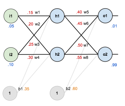
The goal of backpropagation is to optimize the weights so that the neural network can learn how to correctly map arbitrary inputs to outputs.

For the rest of this tutorial we’re going to work with a single training set: given inputs 0.05 and 0.10, we want the neural network to output 0.01 and 0.99.

The Forward Pass

To begin, lets see what the neural network currently predicts given the weights and biases above and inputs of 0.05 and 0.10. To do this we’ll feed those inputs forward though the network.

We figure out the total net input to each hidden layer neuron, squash the total net input using an activation function (here we use the logistic function), then repeat the process with the output layer neurons.

Total net input is also referred to as just net input by some sources.

Here’s how we calculate the total net input for $h_1$ :

$net_{h1} = w_1 * i_1 + w_2 * i_2 + b_1 * 1$

$net_{h1} = 0.15 * 0.05 + 0.2 * 0.1 + 0.35 * 1 = 0.3775$

We then squash it using the logistic function to get the output of $h_1$ :

$out_{h1} = \frac{1}{1+e^{-net_{h1}}} = \frac{1}{1+e^{-0.3775}} = 0.593269992$

Carrying out the same process for $h_2$ we get:

$out_{h2} = 0.596884378$

We repeat this process for the output layer neurons, using the output from the hidden layer neurons as inputs.

Here’s the output for $o_1$ :

$net_{o1} = w_5 * out_{h1} + w_6 * out_{h2} + b_2 * 1$

$net_{o1} = 0.4 * 0.593269992 + 0.45 * 0.596884378 + 0.6 * 1 = 1.105905967$

$out_{o1} = \frac{1}{1+e^{-net_{o1}}} = \frac{1}{1+e^{-1.105905967}} = 0.75136507$

And carrying out the same process for $o_2$ we get:

$out_{o2} = 0.772928465$

Calculating the Total Error

We can now calculate the error for each output neuron using the squared error function and sum them to get the total error:

$E_{total} = \sum \frac{1}{2}(target - output)^{2}$

Some sources refer to the target as the ideal and the output as the actual.

The $\frac{1}{2}$ is included so that exponent is cancelled when we differentiate later on. The result is eventually multiplied by a learning rate anyway so it doesn’t matter that we introduce a constant here [1].

For example, the target output for $o_1$ is 0.01 but the neural network output 0.75136507, therefore its error is:

$E_{o1} = \frac{1}{2}(target_{o1} - out_{o1})^{2} = \frac{1}{2}(0.01 - 0.75136507)^{2} = 0.274811083$

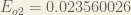
Repeating this process for $o_2$ (remembering that the target is 0.99) we get:

$E_{o2} = 0.023560026$

The total error for the neural network is the sum of these errors:

$E_{total} = E_{o1} + E_{o2} = 0.274811083 + 0.023560026 = 0.298371109$

The Backwards Pass

Our goal with backpropagation is to update each of the weights in the network so that they cause the actual output to be closer the target output, thereby minimizing the error for each output neuron and the network as a whole.

Output Layer

Consider $w_5$ . We want to know how much a change in $w_5$ affects the total error, aka $\frac{\partial E_{total}}{\partial w_{5}}$ .

$\frac{\partial E_{total}}{\partial w_{5}}$ is read as “the partial derivative of $E_{total}$ with respect to $w_{5}$ “. You can also say “the gradient with respect to $w_{5}$ “.

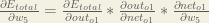
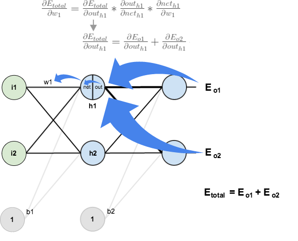
By applying the chain rule we know that:

$\frac{\partial E_{total}}{\partial w_{5}} = \frac{\partial E_{total}}{\partial out_{o1}} * \frac{\partial out_{o1}}{\partial net_{o1}} * \frac{\partial net_{o1}}{\partial w_{5}}$

Visually, here’s what we’re doing:

output_1_backprop (4)

We need to figure out each piece in this equation.

First, how much does the total error change with respect to the output?

$E_{total} = \frac{1}{2}(target_{o1} - out_{o1})^{2} + \frac{1}{2}(target_{o2} - out_{o2})^{2}$

$\frac{\partial E_{total}}{\partial out_{o1}} = 2 * \frac{1}{2}(target_{o1} - out_{o1})^{2 - 1} * -1 + 0$

$\frac{\partial E_{total}}{\partial out_{o1}} = -(target_{o1} - out_{o1}) = -(0.01 - 0.75136507) = 0.74136507$

$-(target - out)$ is sometimes expressed as $out - target$

When we take the partial derivative of the total error with respect to $out_{o1}$ , the quantity $\frac{1}{2}(target_{o2} - out_{o2})^{2}$ becomes zero because $out_{o1}$ does not affect it which means we’re taking the derivative of a constant which is zero.

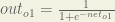
Next, how much does the output of $o_1$ change with respect to its total net input?

The partial derivative of the logistic function is the output multiplied by 1 minus the output:

$out_{o1} = \frac{1}{1+e^{-net_{o1}}}$

$\frac{\partial out_{o1}}{\partial net_{o1}} = out_{o1}(1 - out_{o1}) = 0.75136507(1 - 0.75136507) = 0.186815602$

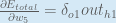
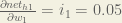
Finally, how much does the total net input of $o1$ change with respect to $w_5$ ?

$net_{o1} = w_5 * out_{h1} + w_6 * out_{h2} + b_2 * 1$

$\frac{\partial net_{o1}}{\partial w_{5}} = 1 * out_{h1} * w_5^{(1 - 1)} + 0 + 0 = out_{h1} = 0.593269992$

Putting it all together:

$\frac{\partial E_{total}}{\partial w_{5}} = \frac{\partial E_{total}}{\partial out_{o1}} * \frac{\partial out_{o1}}{\partial net_{o1}} * \frac{\partial net_{o1}}{\partial w_{5}}$

$\frac{\partial E_{total}}{\partial w_{5}} = 0.74136507 * 0.186815602 * 0.593269992 = 0.082167041$

You’ll often see this calculation combined in the form of the delta rule:

$\frac{\partial E_{total}}{\partial w_{5}} = -(target_{o1} - out_{o1}) * out_{o1}(1 - out_{o1}) * out_{h1}$

Alternatively, we have $\frac{\partial E_{total}}{\partial out_{o1}}$ and $\frac{\partial out_{o1}}{\partial net_{o1}}$ which can be written as $\frac{\partial E_{total}}{\partial net_{o1}}$ , aka $\delta_{o1}$ (the Greek letter delta) aka the node delta. We can use this to rewrite the calculation above:

$\delta_{o1} = \frac{\partial E_{total}}{\partial out_{o1}} * \frac{\partial out_{o1}}{\partial net_{o1}} = \frac{\partial E_{total}}{\partial net_{o1}}$

$\delta_{o1} = -(target_{o1} - out_{o1}) * out_{o1}(1 - out_{o1})$

Therefore:

$\frac{\partial E_{total}}{\partial w_{5}} = \delta_{o1} out_{h1}$

Some sources extract the negative sign from $\delta$ so it would be written as:

$\frac{\partial E_{total}}{\partial w_{5}} = -\delta_{o1} out_{h1}$

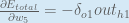
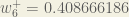
To decrease the error, we then subtract this value from the current weight (optionally multiplied by some learning rate, eta, which we’ll set to 0.5):

$w_5^{+} = w_5 - \eta * \frac{\partial E_{total}}{\partial w_{5}} = 0.4 - 0.5 * 0.082167041 = 0.35891648$

Some sources use $\alpha$ (alpha) to represent the learning rate, others use $\eta$ (eta), and others even use $\epsilon$ (epsilon).

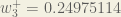
We can repeat this process to get the new weights $w_6$ , $w_7$ , and $w_8$ :

$w_6^{+} = 0.408666186$

$w_7^{+} = 0.511301270$

$w_8^{+} = 0.561370121$

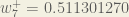
We perform the actual updates in the neural network after we have the new weights leading into the hidden layer neurons (ie, we use the original weights, not the updated weights, when we continue the backpropagation algorithm below).

Hidden Layer

Next, we’ll continue the backwards pass by calculating new values for $w_1$ , $w_2$ , $w_3$ , and $w_4$ .

Big picture, here’s what we need to figure out:

$\frac{\partial E_{total}}{\partial w_{1}} = \frac{\partial E_{total}}{\partial out_{h1}} * \frac{\partial out_{h1}}{\partial net_{h1}} * \frac{\partial net_{h1}}{\partial w_{1}}$

Visually:

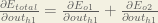
We’re going to use a similar process as we did for the output layer, but slightly different to account for the fact that the output of each hidden layer neuron contributes to the output (and therefore error) of multiple output neurons. We know that $out_{h1}$ affects both $out_{o1}$ and $out_{o2}$ therefore the $\frac{\partial E_{total}}{\partial out_{h1}}$ needs to take into consideration its effect on the both output neurons:

$\frac{\partial E_{total}}{\partial out_{h1}} = \frac{\partial E_{o1}}{\partial out_{h1}} + \frac{\partial E_{o2}}{\partial out_{h1}}$

Starting with $\frac{\partial E_{o1}}{\partial out_{h1}}$ :

$\frac{\partial E_{o1}}{\partial out_{h1}} = \frac{\partial E_{o1}}{\partial net_{o1}} * \frac{\partial net_{o1}}{\partial out_{h1}}$

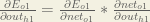
We can calculate $\frac{\partial E_{o1}}{\partial net_{o1}}$ using values we calculated earlier:

$\frac{\partial E_{o1}}{\partial net_{o1}} = \frac{\partial E_{o1}}{\partial out_{o1}} * \frac{\partial out_{o1}}{\partial net_{o1}} = 0.74136507 * 0.186815602 = 0.138498562$

And $\frac{\partial net_{o1}}{\partial out_{h1}}$ is equal to $w_5$ :

$net_{o1} = w_5 * out_{h1} + w_6 * out_{h2} + b_2 * 1$

$\frac{\partial net_{o1}}{\partial out_{h1}} = w_5 = 0.40$

Plugging them in:

$\frac{\partial E_{o1}}{\partial out_{h1}} = \frac{\partial E_{o1}}{\partial net_{o1}} * \frac{\partial net_{o1}}{\partial out_{h1}} = 0.138498562 * 0.40 = 0.055399425$

Following the same process for $\frac{\partial E_{o2}}{\partial out_{h1}}$ , we get:

$\frac{\partial E_{o2}}{\partial out_{h1}} = -0.019049119$

Therefore:

$\frac{\partial E_{total}}{\partial out_{h1}} = \frac{\partial E_{o1}}{\partial out_{h1}} + \frac{\partial E_{o2}}{\partial out_{h1}} = 0.055399425 + -0.019049119 = 0.036350306$

Now that we have $\frac{\partial E_{total}}{\partial out_{h1}}$ , we need to figure out $\frac{\partial out_{h1}}{\partial net_{h1}}$ and then $\frac{\partial net_{h1}}{\partial w}$ for each weight:

$out_{h1} = \frac{1}{1+e^{-net_{h1}}}$

$\frac{\partial out_{h1}}{\partial net_{h1}} = out_{h1}(1 - out_{h1}) = 0.59326999(1 - 0.59326999 ) = 0.241300709$

We calculate the partial derivative of the total net input to $h_1$ with respect to $w_1$ the same as we did for the output neuron:

$net_{h1} = w_1 * i_1 + w_3 * i_2 + b_1 * 1$

$\frac{\partial net_{h1}}{\partial w_1} = i_1 = 0.05$

Putting it all together:

$\frac{\partial E_{total}}{\partial w_{1}} = \frac{\partial E_{total}}{\partial out_{h1}} * \frac{\partial out_{h1}}{\partial net_{h1}} * \frac{\partial net_{h1}}{\partial w_{1}}$

$\frac{\partial E_{total}}{\partial w_{1}} = 0.036350306 * 0.241300709 * 0.05 = 0.000438568$

You might also see this written as:

$\frac{\partial E_{total}}{\partial w_{1}} = (\sum\limits_{o}{\frac{\partial E_{total}}{\partial out_{o}} * \frac{\partial out_{o}}{\partial net_{o}} * \frac{\partial net_{o}}{\partial out_{h1}}}) * \frac{\partial out_{h1}}{\partial net_{h1}} * \frac{\partial net_{h1}}{\partial w_{1}}$

$\frac{\partial E_{total}}{\partial w_{1}} = (\sum\limits_{o}{\delta_{o} * w_{ho}}) * out_{h1}(1 - out_{h1}) * i_{1}$

$\frac{\partial E_{total}}{\partial w_{1}} = \delta_{h1}i_{1}$

We can now update $w_1$ :

$w_1^{+} = w_1 - \eta * \frac{\partial E_{total}}{\partial w_{1}} = 0.15 - 0.5 * 0.000438568 = 0.149780716$

Repeating this for $w_2$ , $w_3$ , and $w_4$

$w_2^{+} = 0.19956143$

$w_3^{+} = 0.24975114$

$w_4^{+} = 0.29950229$

Finally, we’ve updated all of our weights! When we fed forward the 0.05 and 0.1 inputs originally, the error on the network was 0.298371109. After this first round of backpropagation, the total error is now down to 0.291027924. It might not seem like much, but after repeating this process 10,000 times, for example, the error plummets to 0.0000351085. At this point, when we feed forward 0.05 and 0.1, the two outputs neurons generate 0.015912196 (vs 0.01 target) and 0.984065734 (vs 0.99 target).

If you’ve made it this far and found any errors in any of the above or can think of any ways to make it clearer for future readers, don’t hesitate to drop me a note. Thanks!

And while I have you…

In addition to dabbling in data science, I run Preceden timeline maker, the best timeline maker software on the web. If you ever need to create a high level timeline or roadmap to get organized or align your team, Preceden is a great option.

1,042 thoughts on “A Step by Step Backpropagation Example”

Machine Learning by Andrew Ng week 5 ( Summary ) - Jacob is studying on programming
NIkesh says:

April 22, 2019 at 5:11 am

Superb Explaination

Reply
- krishna says:
  
  December 18, 2019 at 1:45 am
  
  I m not getting if same inputs need to regenerate why we are putting hidden layers ,whats is the purpose?
  
  Reply
Chaitra says:

April 23, 2019 at 10:51 am

just awesome explanation…!!

Reply
Mattie says:

April 26, 2019 at 2:34 pm

Took a pen and paper and really enjoyed this. Thanks!

Reply
Cat says:

April 29, 2019 at 11:51 am

This is simply the best explanation I have found for back propagation
Love how you broke everything down!!

Reply
Saheli Mahapatra says:

April 29, 2019 at 10:33 pm

Here is another very nice tutorial with step by step Mathematical explanation and full coding.

http://www.adeveloperdiary.com/data-science/machine-learning/understand-and-implement-the-backpropagation-algorithm-from-scratch-in-python/

Reply
- Syed Mohsin Bukhari says:
  
  July 15, 2019 at 7:00 am
  
  This link has awesome description of backprop. Thanks!
  
  Reply
Charles Yin says:

April 30, 2019 at 2:20 pm

This is the best tutorial on neural work! All textbooks should be written like this. Thank you very much!

Reply
Ava Trimble says:

May 2, 2019 at 12:20 pm

This really was the greatest explanation! Love it. Thanks

Reply
Andrew Bannerman says:

May 7, 2019 at 10:26 pm

Great! Thanks for the walk through! When using different activation functions…. during back propogation we just need to use the derivative of the activation function yes?

Reply
Tony says:

May 8, 2019 at 2:28 am

Teaching is an art! Good Post!

Reply
Nūr Al-Dīn says:

June 10, 2019 at 1:54 pm

Thank you very very very useful topic

Reply
Ashutosh Nayak says:

June 19, 2019 at 4:07 pm

Best explanation for back propagation with clear steps..thanks a lot…

Reply
Anthony says:

July 19, 2019 at 3:50 pm

This is a gem! Thanks so much, Matt! You made me understand in an hour what a semester in grad school failed to do!

Reply
Dont want to give says:

July 23, 2019 at 9:57 am

Such a wanderful and simple explanation

Reply
Jagan Mohan says:

August 8, 2019 at 4:53 pm

Goshhhh….. I am so happy I came across this post. Such a clean way of explanation. Thanks Matt.

Reply
amaury L says:

August 11, 2019 at 3:36 pm

Amazing article, can’t recommend enough ! Not ashamed to cover the math step by step which I am sure not every teacher is always willing to do. Understand it once and the rest will come with it.

Reply
yoliax says:

August 27, 2019 at 3:21 am

Thank you very much, you are artist on deep learing！

Reply
Partha Sarathi says:

September 3, 2019 at 7:31 am

Was looking for exactly this kind of a blog! Thanks!!!

Reply
ryan reza fadillah says:

September 12, 2019 at 5:04 am

wow its amazing

Reply
Mykel Stone says:

September 13, 2019 at 4:43 pm

I just wanted to comment that this blog post has served me well for the last 4 years. I mess with neural networks as a hobby and while I mainly create art pieces that use the chaotic dynamics inherent in these networks, sometimes I like to play around with making something that can learn and this is my go-to read for remembering how to do backpropagation. It saves me so much time! So I’d just like to personally say thank you.

Reply
- Mazur says:
  
  September 13, 2019 at 9:00 pm
  
  Appreciate you saying so!
  
  Reply
Leo says:

September 16, 2019 at 6:01 am

Excellent explanation !

Reply
dikibhuyan says:

September 26, 2019 at 12:04 pm

Don’t you think the hidden nodes should have different bias values? You’re using the same values for hidden nodes on the same layer.

Reply
- Aryan says:
  
  December 5, 2019 at 7:23 am
  
  I have the same doubt! It’s a pity the author isn’t replying. I suppose he must’ve done it for the sake of simplicity but that would defeat the purpose of the article, wouldn’t it? Maybe as an empirical rule the biases for a layer are to be initialized as the same value?
  
  Reply
  - Noah says:
    
    January 6, 2020 at 8:17 pm
    
    I’m betting you just use the chain rule that he uses throughout and the summation that he uses for the hidden layers. Modifying what he says: “We know that b_{2} affects both out_{o1} and out_{o2} therefore the \frac{\partial E_{total}}{\partial b_{2}} needs to take into consideration its effect on the both output neurons”
    
    Reply
Carlos says:

October 30, 2019 at 3:50 am

What about bias values?

Reply
Arun M says:

October 30, 2019 at 1:35 pm

Great material! Thank you so much for your effort! Your idea of plugging numbers into the equation was a great aid in developing understanding and intuition behind this. Will read this many times over until required.

Reply
ANJANA says:

November 7, 2019 at 5:40 am

Thank you sir !!

Reply
Hannah Her. says:

November 7, 2019 at 6:25 am

This is an awesome tutorial, thank you very much. I only struggle at one point, namely the Backward Pass, Output Layer. You write

E_Total = 1/2 (target_o1 – out_o1)^2 + 1/2 (target_o1 – out_o2)^2

That is clear to me. But then the next line reads:

φE_Total/φout_o1 = 2 * 1/2 (target_o1 – out_o1)^2-1 * -1 +0 <<– Where is the '-1' coming from? I spend an hour trying to understand it, but I just don't. Any help would be greatly appreciated.

Hannah

Reply
- MinimalArchitect says:
  
  December 21, 2019 at 6:15 pm
  
  If you use the correct partial-derivative without the -1, you would need to add the new weight onto the old one (not subtract them), so it’s a unexplained side-product that everyone seems to use.
  
  Reply
- Afer Ventus says:
  
  December 29, 2019 at 1:59 am
  
  1/2 (target_o1 – out_o1)^2
  the derivative of this function states that:
  a) the exponent becomes the multiplier, so:
  1/2 (target_o1 – out_o1)^2
  becomes
  2 * 1/2 (target_o1 – out_o1)^2
  
  b) subtract 1 from the exponent, so:
  2 * 1/2 (target_o1 – out_o1)^2
  becomes
  2 * 1/2 (target_o1 – out_o1)^2-1
  
  c) the inner function g(x) = out_o1, so:
  2 * 1/2 (target_o1 – x)^2-1
  
  d) the “x” has 1 as exponent. The derivative states that it should be subtracted by 1, so:
  2 * 1/2 (target_o1 – x^1-1)^2-1
  which results in
  2 * 1/2 (target_o1 – x^0)^2-1
  
  e) every number powered by zero becomes 1, so:
  2 * 1/2 (target_o1 – 1)^2-1
  
  f) it is a composite function, so applying the chain rule:
  f′(g(x))⋅g′(x)
  
  g'(x) = -1
  
  the -1 is g'(x). The remaining before it is f'(g(x))
  
  Reply
- luqing says:
  
  October 28, 2020 at 11:55 pm
  
  The -1 comes from the derivative of -out_o1 within the parenthesis.
  
  Reply
Martti says:

November 13, 2019 at 9:07 am

Excellent story about backpropagation. I tried to make a C++ implementation. I managed to do the same numeric values for the weights. However there is no lines about the bias adjusting. Can biases b1 and b2 adjusted like weights, where the inputs always 1.0 ?
Thanks

Reply
MANUEL OMAR OLGUIN HERNANDEZ says:

November 19, 2019 at 12:08 pm

Thanks for your explanation, is good, however, I can’t see how Bias could adjust. could you help us. Tks

Reply
gg1101 says:

November 20, 2019 at 6:40 pm

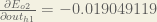
PLEASE, answer me, the term d(E_o2)/d(out_h1) should be -0.02229036407211166… check pleaseeee
Anyway, best explanation on internet

Reply
Ravi says:

December 4, 2019 at 11:41 am

This is a really nice explanation. Good job.

Reply
asdf says:

December 6, 2019 at 11:00 pm

Bless your heart… Thank you.

Reply
James says:

January 2, 2020 at 10:28 pm

Excellent explanation! Would love to see the calculations followed through for the biases too.

Reply
Ishan Dindorkar says:

January 6, 2020 at 4:48 am

Thank you so much for writing this awesome blog. I greatly appreciate your efforts

Reply
vinay says:

January 9, 2020 at 9:55 pm

I am unable to understand net_o1 = w_5 * out_h1 + w_6 * out_h2+ b_2 * 1. how does the derivative translate into 1 * out_h1 * w_5^(1 – 1) + 0 + 0 = out_h1 = 0.593269992, from where did w_5^(1-1) come from shouldnt it just be 1 * out_h1 * w_5^(1 – 1)

Reply
Vinay Vernekar says:

January 9, 2020 at 10:47 pm

I am unable to understand net_o1 = w_5 * out_h1 + w_6 * out_h2+ b_2 * 1. how does the derivative translate into1 * out_h1 * w_5^(1 – 1) + 0 + 0 = out_h1 = 0.593269992, from where did w_5^(1-1) come from shouldnt it just be 1 * out_h1 * w_5^(1 – 1)

Reply
cthulhuu says:

January 30, 2020 at 5:02 am

Best explanation i’ve ever seen.

Reply
Joe Scanlan says:

May 16, 2020 at 12:42 pm

Hi Matt
This review is one of the best I have ever seen. Thanks for your efforts.

Joe Scanlan email: scangang5@aol.com

Reply
Fernando Arbe says:

May 19, 2020 at 1:05 am

Congratulations. Really a good tutorial. Just what I was looking for.

Reply
Peter says:

May 21, 2020 at 7:12 am

Man, you saved my life. I was looking for a proper, but easy to understand backprop tutorial. God bless you.

Reply
Homer says:

May 22, 2020 at 6:34 pm

Bravo! The most readable demonstration of how back propagation actually works so far!

Reply
Hyeongcheol Park says:

May 30, 2020 at 3:52 am

holly cow really helpful! Thanks so much!

Reply
Andrej Noskaj says:

June 13, 2020 at 4:44 pm

Can anyone please explain how did he get the value -0.019049119? I always get something different.

Reply
Praveen says:

June 14, 2020 at 6:20 am

Best explanation with simple example!
Cheers

Reply
Sergius says:

June 15, 2020 at 2:36 am

why for updating w7 & w8 you put negative (-) on “the gradient with respect to w7”?
I have no idea about this because at the first you didnt put (-) for updating w5 & w6. it is change my w7 & w8 updating result if I don’t use that (-)

Reply
Hyperparameters for Classifying Images with Convolutional Neural Networks – Part 1 – Learning Rate – Ironman John
Hyperparameters for Classifying Images with Convolutional Neural Networks – Part 2 – Batch Size – Ironman John
ENG. EDISON says:

June 18, 2020 at 5:44 am

That explanations needs a bottle of champagne,well explained.

Reply
shahomaghdeed@gmail.com says:

June 20, 2020 at 4:33 am

This is the best tutorial on neural work! All textbooks should be written like this. Thank you very much!

Reply
shaho maghdid says:

June 20, 2020 at 4:36 am

bravo

Reply
How is a neural network - Prog.world